A&A 489, 23-35 (2008)
DOI: 10.1051/0004-6361:200809646
M. Limousin1,2 - J. Richard3 - J.-P. Kneib4 - H. Brink2 - R. Pelló5 - E. Jullo4 - H. Tu6,7,8 - J. Sommer-Larsen9,2 - E. Egami10 - M. J. Micha![]() owski2 - R. Cabanac1 - D. P. Stark3
owski2 - R. Cabanac1 - D. P. Stark3
1 - Laboratoire d'Astrophysique de Toulouse-Tarbes, Université de Toulouse, CNRS, 57 avenue d'Azereix, 65000 Tarbes, France
2 - Dark Cosmology Centre, Niels Bohr Institute, University of Copenhagen,
Juliane Maries Vej 30, 2100 Copenhagen, Denmark
3 -
Department of Astronomy, California Institute of Technology, 105-24, Pasadena, CA91125, USA
4 - Laboratoire d'Astrophysique de Marseille, CNRS-Université de Provence, 38 rue Frédéric Joliot-Curie, 13388 Marseille Cedex 13, France
5 -
Laboratoire d'Astrophysique de Toulouse-Tarbes, Université de Toulouse, CNRS,
14 avenue Edouard Belin, 31400 Toulouse, France
6 - Physics Department, Shanghai Normal University, 100 Guilin Road, Shanghai 200234, PR China
7 - Institut d'Astrophysique de Paris, CNRS, 98bis Bvd Arago, 75014 Paris, France
8 - Shanghai Astronomical Observatory, 80 Nandan Road, Shanghai 200030, PR China
9 - Excellence Cluster Universe, Technische Universität München, Boltz-manstr. 2, 85748 Garching, Germany
10 - Steward Observatory, University of Arizona, 933 North Cherry Avenue, Tucson, AZ 85721, USA
Received 25 February 2008 / Accepted 12 July 2008
Abstract
Properties of dark matter haloes can be probed observationally and numerically, and comparing both approaches provides ways to constrain cosmological models.
When it comes to the inner part of galaxy cluster scale haloes, interaction between the baryonic and the dark matter component is an important issue that is far from being fully understood.
With this work, we aim to initiate a program coupling observational and numerical studies to
probe the inner part of galaxy clusters. In this article, we apply strong lensing techniques on Abell 1703, a massive X-ray luminous galaxy cluster at z=0.28. Our analysis is based on imaging data from both the space and ground in 8 bands, complemented by a spectroscopic survey.
Abell 1703 is rather circular from the general shape of its multiply imaged systems and is dominated by a giant elliptical cD galaxy in its centre. This cluster exhibits a remarkable bright
central ring
formed by 4 images at
![]() only 5-13
only 5-13
![]() away from the cD centre. This unique feature offers a rare lensing constrain for probing the central mass distribution.
The stellar contribution from the cD galaxy (
away from the cD centre. This unique feature offers a rare lensing constrain for probing the central mass distribution.
The stellar contribution from the cD galaxy (
![]() within 30 kpc) is accounted for in our parametric mass modelling, and the underlying
smooth dark matter component distribution is described using a generalized NFW profile parametrized with a central logarithmic slope
within 30 kpc) is accounted for in our parametric mass modelling, and the underlying
smooth dark matter component distribution is described using a generalized NFW profile parametrized with a central logarithmic slope ![]() .
The rms of our mass model in the image plane is equal to 1.4
.
The rms of our mass model in the image plane is equal to 1.4
![]() .
We find that within the range where observational constraints are present
(from
.
We find that within the range where observational constraints are present
(from ![]() 20 kpc to
20 kpc to ![]() 210 kpc),
210 kpc), ![]() is
equal to
1.09+0.05-0.11 (3
is
equal to
1.09+0.05-0.11 (3![]() confidence level).
The concentration parameter is equal to
confidence level).
The concentration parameter is equal to
![]() ,
and the scale radius is constrained to be larger than the region where observational constraints are available (
,
and the scale radius is constrained to be larger than the region where observational constraints are available (
![]() kpc). The 2D mass is equal to
kpc). The 2D mass is equal to
![]() .
However, we cannot draw any conclusions on cosmological models at this point since we lack results from realistic numerical simulations containing baryons to make a proper comparison. We advocate the need for a large sample of well observed (and well constrained) and simulated unimodal relaxed galaxy clusters in order to make reliable comparisons and to potentially provide a test of cosmological models.
.
However, we cannot draw any conclusions on cosmological models at this point since we lack results from realistic numerical simulations containing baryons to make a proper comparison. We advocate the need for a large sample of well observed (and well constrained) and simulated unimodal relaxed galaxy clusters in order to make reliable comparisons and to potentially provide a test of cosmological models.
Key words: gravitational lensing - galaxies: clusters: individual: Abell 1703 - dark matter
Large N-body cosmological simulations have been carried out for a decade, with the goal of making statistical predictions on dark matter (DM) halo properties.
Because of numerical issues, most of these large cosmological simulations contain dark matter particles only. They all reliably predict that the 3D density profile
![]() should fall as r-3 beyond what is usually called the scale radius. Observations have confirmed these predictions (e.g. Kneib et al. 2003; Pointecouteau et al. 2005; Mandelbaum et al. 2008).
This agreement is likely to be connected with the fact that at large radius, the density profile of a galaxy cluster is dark matter dominated and the influence of baryons can be neglected. On smaller scales, if we parametrize the 3D density profile of the DM using a cuspy profile
should fall as r-3 beyond what is usually called the scale radius. Observations have confirmed these predictions (e.g. Kneib et al. 2003; Pointecouteau et al. 2005; Mandelbaum et al. 2008).
This agreement is likely to be connected with the fact that at large radius, the density profile of a galaxy cluster is dark matter dominated and the influence of baryons can be neglected. On smaller scales, if we parametrize the 3D density profile of the DM using a cuspy profile
![]() ;
dark matter only simulations predict a logarithmic slope
;
dark matter only simulations predict a logarithmic slope
![]() -1.5 for
-1.5 for
![]() .
The exact value of the central slope and its universality is debated (Navarro et al. 1997; Moore et al. 1998; Ghigna et al. 2000; Gao et al. 2008; Ricotti 2003; Navarro et al. 2004).
From the theoretical point of view, the logarithmic slope of DM haloes is predicted to be
.
The exact value of the central slope and its universality is debated (Navarro et al. 1997; Moore et al. 1998; Ghigna et al. 2000; Gao et al. 2008; Ricotti 2003; Navarro et al. 2004).
From the theoretical point of view, the logarithmic slope of DM haloes is predicted to be
![]() (Austin et al. 2005; Hansen & Stadel 2006). Although this debate is of some interest, these dark matter only studies and their predictions do not help much to make comparison with observations. Indeed, observing the central part (i.e. the inner
(Austin et al. 2005; Hansen & Stadel 2006). Although this debate is of some interest, these dark matter only studies and their predictions do not help much to make comparison with observations. Indeed, observing the central part (i.e. the inner ![]() 500 kpc) of a galaxy cluster at any wavelength reveals the presence of baryons (in the forms of stars and X-ray hot gas).
Thus any attempt to compare observations to simulations in the centre of galaxy clusters has to be made with numerical simulations (or calculations) taking into account the baryonic component and its associated physics.
500 kpc) of a galaxy cluster at any wavelength reveals the presence of baryons (in the forms of stars and X-ray hot gas).
Thus any attempt to compare observations to simulations in the centre of galaxy clusters has to be made with numerical simulations (or calculations) taking into account the baryonic component and its associated physics.
Efforts are currently developed on the numerical side in order to account for the presence of baryons (e.g. the Horizon![]() simulation). In practice, our understanding of the baryonic physics is poor, and the exact interplay between dark matter and baryon is far from understood. For example, due to the overcooling problem, numerical simulations predict blue central brightest cluster galaxies which are not always observed.
Different effects do compete when it comes to the central slope of the density profile: the cooling of gas in the centre of dark matter haloes is expected to lead to a more concentrated dark matter distribution (the so-called adiabatic contraction, see Blumenthal et al. 1986; Gustafsson et al. 2006; Gnedin et al. 2004). On the other hand, dynamical friction heating of massive galaxies against the diffuse cluster dark matter can flatten the slope of the DM density profile (Ma & Boylan-Kolchin 2004; Nipoti et al. 2003,2004; El-Zant et al. 2001),
and this effect could even dominate over adiabatic contraction (El-Zant et al. 2004).
Note also that the properties of the inner part of simulated galaxy clusters (even in dark matter only simulations) can depend significantly on initial conditions as demonstrated in Kazantzidis et al. (2004). To summarize, no coherent picture has yet emerged from N-body simulations when it comes to the shape of the inner density profile of structures; this problem is a difficult one and the answer is likely not to be unique but may depend on the physical properties of the structures and their formation history.
simulation). In practice, our understanding of the baryonic physics is poor, and the exact interplay between dark matter and baryon is far from understood. For example, due to the overcooling problem, numerical simulations predict blue central brightest cluster galaxies which are not always observed.
Different effects do compete when it comes to the central slope of the density profile: the cooling of gas in the centre of dark matter haloes is expected to lead to a more concentrated dark matter distribution (the so-called adiabatic contraction, see Blumenthal et al. 1986; Gustafsson et al. 2006; Gnedin et al. 2004). On the other hand, dynamical friction heating of massive galaxies against the diffuse cluster dark matter can flatten the slope of the DM density profile (Ma & Boylan-Kolchin 2004; Nipoti et al. 2003,2004; El-Zant et al. 2001),
and this effect could even dominate over adiabatic contraction (El-Zant et al. 2004).
Note also that the properties of the inner part of simulated galaxy clusters (even in dark matter only simulations) can depend significantly on initial conditions as demonstrated in Kazantzidis et al. (2004). To summarize, no coherent picture has yet emerged from N-body simulations when it comes to the shape of the inner density profile of structures; this problem is a difficult one and the answer is likely not to be unique but may depend on the physical properties of the structures and their formation history.
On the observational side, efforts have been put on probing the central slope ![]() of the underlying dark matter distribution. These analyses have led to wide-ranging results, whatever the method used: X-ray (Zappacosta et al. 2006; Ettori et al. 2002; Arabadjis et al. 2002; Lewis et al. 2003);
lensing (Bradac et al. 2007; Gavazzi et al. 2003; Dahle et al. 2003; Tyson et al. 1998; Gavazzi 2005; Smith et al. 2001; Sand et al. 2004,2008,2002) or dynamics (Biviano & Salucci 2006; Kelson et al. 2002). This highlight the difficulty of such studies and the possible large scatter in the value of
of the underlying dark matter distribution. These analyses have led to wide-ranging results, whatever the method used: X-ray (Zappacosta et al. 2006; Ettori et al. 2002; Arabadjis et al. 2002; Lewis et al. 2003);
lensing (Bradac et al. 2007; Gavazzi et al. 2003; Dahle et al. 2003; Tyson et al. 1998; Gavazzi 2005; Smith et al. 2001; Sand et al. 2004,2008,2002) or dynamics (Biviano & Salucci 2006; Kelson et al. 2002). This highlight the difficulty of such studies and the possible large scatter in the value of ![]() from one cluster to another.
from one cluster to another.
To summarize, we need to probe observationally and numerically the behaviour of the underlying dark matter distribution (i.e. after the baryonic component has been separated from the dark matter component) in the central parts of galaxy clusters.
The main difficulties are: i) observationally, to be able to disentangle the baryonic component and the underlying dark matter distribution; ii) numerically, to implement the baryonic physics into the simulations; iii) then to compare both approaches in a consistent way. These issues are far beyond the scope of this article, but they are likely to provide an interesting test of the ![]() CDM scenario in the future.
CDM scenario in the future.
In this work, we aim to probe observationally the central (i.e. from
![]() (
(![]() 20 kpc) up to
20 kpc) up to
![]() (
(![]() 200 kpc) from the centre) density profile of a massive cluster lens. Our main goal is to measure the slope of the inner underlying dark matter distribution within this radius. In practice, we apply strong lensing techniques on galaxy cluster Abell 1703,
a massive z=0.28 (Allen et al. 1992) X-ray cluster with a luminosity
200 kpc) from the centre) density profile of a massive cluster lens. Our main goal is to measure the slope of the inner underlying dark matter distribution within this radius. In practice, we apply strong lensing techniques on galaxy cluster Abell 1703,
a massive z=0.28 (Allen et al. 1992) X-ray cluster with a luminosity
![]() erg s-1 (Böhringer et al. 2000).
It is very well suited for the analysis we want to perform for the following reasons:
erg s-1 (Böhringer et al. 2000).
It is very well suited for the analysis we want to perform for the following reasons:
All our results are scaled to the flat, ![]() CDM cosmology with
CDM cosmology with
![]() and a Hubble constant
and a Hubble constant
![]() km s-1 Mpc-1. In such a cosmology, at z=0.28,
km s-1 Mpc-1. In such a cosmology, at z=0.28,
![]() corresponds to 4.244 kpc. All the figures of the cluster are aligned with WCS coordinates, i.e. north is up, east is left. The reference centre of our analysis is fixed at the cD centre: RA = 13:15:05.276, Dec = +51:49:02.85 (J 2000.0). Magnitudes are given in the AB system.
corresponds to 4.244 kpc. All the figures of the cluster are aligned with WCS coordinates, i.e. north is up, east is left. The reference centre of our analysis is fixed at the cD centre: RA = 13:15:05.276, Dec = +51:49:02.85 (J 2000.0). Magnitudes are given in the AB system.
![\begin{figure}
\par\includegraphics[height=22cm,width=18cm]{9646fig1.ps}\end{figure}](/articles/aa/full/2008/37/aa09646-08/img44.gif) |
Figure 1:
Colour image of Abell 1703 from F850W, F625W and F475W observations (Stott 2007). North is up, east is left. Size of the field of view is equal to
|
| Open with DEXTER | |
The multiwavelength ACS data have been used to construct colour images of Abell 1703 in order to identify the multiply imaged systems. In addition to the 6 ACS bands, we benefited from NICMOS and Subaru data in order to construct spectral energy distributions (SED) and estimate photometric redshifts for the multiple images as well as the stellar mass of the cD galaxy.
![\begin{figure}
\par\includegraphics[height=5.6cm,width=14cm,clip]{9646fig2.ps}\end{figure}](/articles/aa/full/2008/37/aa09646-08/img46.gif) |
Figure 2:
Spectroscopic observation of image 1.1. Left: position of the slit. Right: 1D spectrum. The
|
| Open with DEXTER | |
Table 1: Multiply imaged systems considered in this work.
We used LRIS on Keck I in an attempt to measure a redshift for the brightest component of system 1 (image 1.1). Four exposures
of 900 s were taken on Jan. 29th 2008, under photometric conditions but a poor seeing
(1.4
![]() ), using the 900 lines mm-1 grating blazed at 6320 Å in the red channel of the instrument. This setup covers the wavelength range 5600-7200 Å at a resolution of 2.77 Å and a dispersion of 0.83 Å per pixel. The spectrum has been reduced with standard IRAF procedures for bias correction, flat-fielding, sky subtraction and distortion correction, in that order. We used the numerous sky lines in this region for the wavelength calibration and observation of the standard star Feige 92 for the flux calibration.
), using the 900 lines mm-1 grating blazed at 6320 Å in the red channel of the instrument. This setup covers the wavelength range 5600-7200 Å at a resolution of 2.77 Å and a dispersion of 0.83 Å per pixel. The spectrum has been reduced with standard IRAF procedures for bias correction, flat-fielding, sky subtraction and distortion correction, in that order. We used the numerous sky lines in this region for the wavelength calibration and observation of the standard star Feige 92 for the flux calibration.
We detected a bright doublet of emission lines, centred at 7036 and 7041 Å respectively, which we interpret as
![]() at
at
![]() without any ambiguity, the doublet being easily separated by 5
without any ambiguity, the doublet being easily separated by 5 ![]() at this resolution (Fig. 2). The spectroscopic redshift is in agreement with our photometric redshift estimate of
at this resolution (Fig. 2). The spectroscopic redshift is in agreement with our photometric redshift estimate of
![]() (Table 1).
(Table 1).
We created photometric catalogues combining the multicolour images by running
SExtractor (Bertin & Arnouts 1996) in double image mode. A specific detection image was created by combining all the ACS data after scaling them to the same
background noise level. We used the cD-subtracted images (see Sect. 2.6) for ACS and MOIRCS to prevent any strong photometric contamination in the central
regions, in particular for the measurement of the lensed ring-shape
system (system 1). Photometry was optimized to the small size of the lensed background galaxies, by measuring the flux in a 1.0
![]() diameter aperture. This gives accurate colours in the optical
bands that used the same instrument. We estimated aperture corrections
in the near-infrared by measuring the photometry of 10 isolated bright
point sources in the NICMOS and MOIRCS images, and corrected our
photometric catalogues for this difference.
diameter aperture. This gives accurate colours in the optical
bands that used the same instrument. We estimated aperture corrections
in the near-infrared by measuring the photometry of 10 isolated bright
point sources in the NICMOS and MOIRCS images, and corrected our
photometric catalogues for this difference.
We increased the photometric error bars, usually underestimated by SExtractor, to take into account the effects of drizzling in the reduction of ACS and NICMOS images, following the computations by Casertano et al. (2000). For the MOIRCS images, we measured the pixel-to-pixel background noise from blank regions of sky selected in the original images, and scaled it to the aperture size used in the photometry.
To extract cluster galaxies, we plot the characteristic cluster red sequences (F775W - H) and (F625W - H) in two colour-magnitude diagrams and select the objects lying on both red-sequences as cluster galaxies. This yields 345 early-type cluster galaxies down to F775W=24. For the purpose of the modelling, we will consider only the cluster members whose magnitude is brighter than 21 in the F775W band (in order to save computing time, see Elíasdóttir et al. 2007) and which are located close to some multiply imaged systems. We consider fainter galaxies only if they are located close to some multiple images since they can locally perturb the lensing configuration (Meneghetti et al. 2007a). This yields 45 galaxy scale perturbers.
We ran the photometric redshift code HyperZ (Bolzonella et al. 2000) on the multi-band photometric catalogues, in order to get a redshift estimate for all the multiple images identified in the field. This program performs a minimization procedure between the spectral energy distribution of each object and a library of spectral templates, either empirical (Coleman et al. 1980; Kinney et al. 1996) or from the evolutionary models by Bruzual & Charlot (2003). Note that the NICMOS data we have correspond to a mosaic of four pointings, none of them being centred on the
cD galaxy. It results that the cD galaxy is not fully sampled by the NICMOS data.
Therefore, it cannot be subtracted in the NICMOS image, thus we did not take into
account the F110W filter measurement for all its neighbouring objects, or
for multiple images located at the edges of the NICMOS field of view.
Absolute photometric calibration between the different bands is usually
accurate down to 0.05 mag, we used this value as a minimal value
in the code (this value will be used also for fitting the SED of the cD galaxy in Sect. 2.6). We scanned the following range of parameters: 0.0<z<7.0 for the redshift,
![]() for the reddening, applied on the template spectra with the Calzetti et al. (2000) law observed in starburst galaxies. Optical depth in the Lyman-
for the reddening, applied on the template spectra with the Calzetti et al. (2000) law observed in starburst galaxies. Optical depth in the Lyman-![]() forest followed the Madau (1995) prescription.
forest followed the Madau (1995) prescription.
The results obtained for each multiple image are reported in Table 1, along with the 3![]() error bar estimate given by HyperZ from the redshift probability distribution.
error bar estimate given by HyperZ from the redshift probability distribution.
Abell 1703 exhibits a dominant central giant elliptical galaxy: its stellar contribution to the mass budget in the central part is to be taken properly into account. We worked out some of the cD galaxy properties from the broad band photometry. In particular, we are interested in computing its luminosities in the different filters in order to estimate its stellar mass. Note again that we have not been able to study the cD galaxy in the NICMOS band since the NICMOS data correspond to a mosaic of four pointings, none of them being centred on the cD galaxy.
Table 2: Different observations of Abell 1703 used in this work:instrument, filter and exposure time in seconds.
Table 3: Luminosities and stellar mass to light ratio computed indifferent rest frame filters.
This is comparable (though a bit higher, but note that this galaxy has a very massive stellar population) to typical values of stellar mass to light ratio for giant elliptical galaxies (Gerhard et al. 2001).
Figure 1 shows a colour image of Abell 1703 where we label the multiply imaged systems. We report their positions and photometric redshifts in Table 1. The identification is a difficult step which is done in an iterative fashion: we begin to build a model using the most obvious lensed features. Then this model is used to test and predict possible multiply imaged systems. In total, we use 13 multiply imaged systems in this analysis. It is certain that more systems have to be found within the ACS field that presents many likely blue lensed features.
Here we give some notes on the different systems, and present colour images for each system in Appendix.
![\begin{figure}
\par\includegraphics[height=7cm,width=7cm]{9646fig3.ps}\end{figure}](/articles/aa/full/2008/37/aa09646-08/img124.gif) |
Figure 3:
Integrated luminosity profile of the cD galaxy, in the B band rest frame, for the fit with reddening (solid) and without reddening (dashed), The corresponding mass profile used in the strong lensing analysis is shown as dot-dashed line. Both profiles have the same behaviour for
|
| Open with DEXTER | |
![\begin{figure}
\par\includegraphics[height=8cm,width=6.5cm,angle=-90]{9646fig4.ps}\end{figure}](/articles/aa/full/2008/37/aa09646-08/img125.gif) |
Figure 4:
Results of the SED fitting procedure. Luminosities are computed in an aperture of 7
|
| Open with DEXTER | |
To reconstruct the mass distribution in Abell 1703, we use a parametric method
as implemented in the publicly available LENSTOOL![]() software (Jullo et al. 2007). We use the observational constraints (positions of the multiply imaged systems) to optimize the parameters used to describe the mass distribution: this is what we refer to as optimization procedure. The strong lensing methodology used in this analysis has been described in details in Limousin et al. (2007b). We refer the interested reader to this article for a complete description of our methodology.
software (Jullo et al. 2007). We use the observational constraints (positions of the multiply imaged systems) to optimize the parameters used to describe the mass distribution: this is what we refer to as optimization procedure. The strong lensing methodology used in this analysis has been described in details in Limousin et al. (2007b). We refer the interested reader to this article for a complete description of our methodology.
We describe the mass distribution in Abell 1703 by constructing a two components mass model: the contribution from the dominant central cD galaxy is fixed by its stellar mass, and then the remaining mass is put into an underlying smooth dark matter distribution described using a generalized NFW profile (see Sand et al. 2008, for details on the implementation of the generalized NFW profile into the LENSTOOL code). We also take into account the perturbations associated with the galaxies.
Degeneracies can arise between the two mass components: if too much mass is put into the cD galaxy, then this can lead to a shallower slope of the dark matter halo and vice versa. Therefore, special care has to be taken when modelling the cD galaxy, and such a modelling must be as much as possible
``observationally motivated''. We use a dual Pseudo Isothermal Elliptical Mass Distribution (dPIE, see Elíasdóttir et al. 2007) with no
core radius to describe the cD stellar mass contribution.
This profile is formally the same as the Pseudo Isothermal Elliptical Mass Distribution (PIEMD) profile described in Limousin et al. (2005).
However, as explained in Elíasdóttir et al. (2007) it is not the same as the PIEMD originally defined by Kassiola & Kovner (1993). Therefore we have adopted the new name dPIE to avoid confusion. The position of this mass clump is fixed at (0, 0); the ellipticity and position angle
are set to be the one we measured from the light distribution.
Given this parametrization, the mass of the cD scales as
![]() ,
where the scale radius
,
where the scale radius
![]() is almost equal to the half mass radius, and
is almost equal to the half mass radius, and
![]() is a fiducial velocity dispersion (Elíasdóttir et al. 2007).
The choice of the scale radius will influence the shape of the mass profile.
The smaller the scale radius, the steeper the mass profile.
We choose a scale radius of 25 kpc so that the mass profile is as close as possible to the integrated luminosity profile. As we can see in Fig. 3, the mass profile and the luminosity
profile have the same behaviour for
is a fiducial velocity dispersion (Elíasdóttir et al. 2007).
The choice of the scale radius will influence the shape of the mass profile.
The smaller the scale radius, the steeper the mass profile.
We choose a scale radius of 25 kpc so that the mass profile is as close as possible to the integrated luminosity profile. As we can see in Fig. 3, the mass profile and the luminosity
profile have the same behaviour for
![]() .
Note that 25 kpc is close to the value used by Sand et al. (2008) to describe the cD galaxies in MS 2137 (22 kpc) and Abell 383 (26 kpc), where the same mass profile has been used. The only free parameter describing this cD galaxy is then
.
Note that 25 kpc is close to the value used by Sand et al. (2008) to describe the cD galaxies in MS 2137 (22 kpc) and Abell 383 (26 kpc), where the same mass profile has been used. The only free parameter describing this cD galaxy is then ![]() .
This parameter is allowed to vary in a range that is set by the choice of the scale radius and the estimation of the stellar mass.
.
This parameter is allowed to vary in a range that is set by the choice of the scale radius and the estimation of the stellar mass.
We assume that the dark matter component can be described using a generalized NFW model. Its 3D mass density profile is given by:
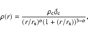 |
(1) |
Note that we have subtracted only the stellar contribution of the cD galaxy in our modelling. This is consistent with the general picture that the dark matter halo of the cluster is also the one of the cD galaxy (see, e.g. Miralda-Escude 1995). We cannot distinguish both haloes.
On top of these two components, we include the brightest cluster members in the optimization (Sect. 2.3). This galaxy scale component is incorporated into the modelling using empirical scaling relations that relate their dynamical parameters (central velocity dispersion and scale radius) to their luminosity, whereas their geometrical parameters (centre, ellipticity, position angle) are set to the one measured from the light distribution (see Limousin et al. 2007b, for details). This galaxy scale component is thus parametrized by only two free parameters, and at the end of the optimization procedure, we get constraints on the parameters for a galaxy of a given (arbitrary) luminosity which corresponds to an observed magnitude mF775W=18.3.
One single galaxy (labeled 852 in our catalogue) is optimized individually, in the sense that some of the parameters describing this galaxy are allowed to vary instead of being fixed by its luminosity. This was necessary to reproduce better the geometrical configuration of some images falling close to this galaxy (systems 3, 7, 8 and 9). In fact, a visual inspection at the image of the cluster shows that this galaxy is very bright and extended (Fig. 1). This galaxy is not representative of the cluster galaxy population, thus the adopted scaling laws might not apply to this object. Moreover, as shown in Appendix, a likely lensed blue feature is coming out from this galaxy, suggesting a massive substructure.
Each parameter is allowed to vary between some limits (priors).
The position of the DM clump was allowed to vary between ![]()
![]() along the X and Y directions. Its ellipticity was forced to be lower than 0.5, since beyond that, the ellipticity as defined in this work for an NFW profile is no longer valid (Golse & Kneib 2002). Its slope
along the X and Y directions. Its ellipticity was forced to be lower than 0.5, since beyond that, the ellipticity as defined in this work for an NFW profile is no longer valid (Golse & Kneib 2002). Its slope ![]() was allowed to vary between 0.2 and 2.0 and its scale radius
was allowed to vary between 0.2 and 2.0 and its scale radius ![]() between
150 and 750 kpc (Dolag et al. 2004; Tasitsiomi et al. 2004). The concentration parameter c200 was allowed to vary between 2.5 and 9, which is large enough to include the expectations from the most recent results from N-body simulations (Neto et al. 2007). The mass of the cD component was forced to be within the range allowed by the stellar mass estimate. Concerning the galaxy scale component, we allowed the velocity dispersion to vary between 150 and 250 km s-1, and the scale radius was forced to be smaller than 70 kpc, since we have evidence both from observations (Natarajan et al. 2002b,a; Geiger & Schneider 1999; Natarajan et al. 1998; Halkola et al. 2007; Limousin et al. 2007a) and from numerical simulations (Limousin et al. 2007c) that dark matter haloes of cluster galaxies are compact due to tidal stripping.
between
150 and 750 kpc (Dolag et al. 2004; Tasitsiomi et al. 2004). The concentration parameter c200 was allowed to vary between 2.5 and 9, which is large enough to include the expectations from the most recent results from N-body simulations (Neto et al. 2007). The mass of the cD component was forced to be within the range allowed by the stellar mass estimate. Concerning the galaxy scale component, we allowed the velocity dispersion to vary between 150 and 250 km s-1, and the scale radius was forced to be smaller than 70 kpc, since we have evidence both from observations (Natarajan et al. 2002b,a; Geiger & Schneider 1999; Natarajan et al. 1998; Halkola et al. 2007; Limousin et al. 2007a) and from numerical simulations (Limousin et al. 2007c) that dark matter haloes of cluster galaxies are compact due to tidal stripping.
Results of the optimization![]() are given in Table 4. The images are well reproduced by our mass model, with an image plane rms equal to 1.4
are given in Table 4. The images are well reproduced by our mass model, with an image plane rms equal to 1.4
![]() (0.2
(0.2
![]() in the source plane).
rms for individual systems are listed in Table 1.
We derive from our model a 2D projected mass within 50
in the source plane).
rms for individual systems are listed in Table 1.
We derive from our model a 2D projected mass within 50
![]() equal to
equal to
![]() .
.
Table 4: Mass model parameters.
We compare the mass and the light distribution in Fig. 6. We find they do compare well, suggesting that light traces mass in Abell 1703. Also shown is the light distribution from the dominant cD galaxy, which is found to be consistent with the one of the overall mass distribution within a few degrees. Moreover, we find the centre of the DM halo to be coincident with the centre of the cD galaxy.
At first approximation, these facts suggest that Abell 1703 is a relaxed unimodal cluster. This hypothesis should be investigated further, in particular with precise X-ray observations since we expect the X-ray emission to be centred on the cD galaxy, and to present a low ellipticity.
Besides, we can draw a line from the southern part of the ACS field
up to its northern part that pass through the cD galaxy and that connects very bright galaxies, much brighter than the overall galaxy population (Fig. 1). Interestingly, when looking at Abell 1703 on much larger scales from SDSS imaging (which size is
![]() ), the whole cluster galaxy population looks rather homogeneous, with no very luminous galaxies as we can observe along this filamentary structure.
In the south of the ACS field, this structure seem to have an influence on the formation of the giant arc, breaking its symmetry (Appendix). The perturbation associated with the northern part of this structure is more obvious to detect. Indeed, the formation of systems 3, 7, 8, and 9 (both their existence and their geometrical configuration) is connected with this extra mass component. Moreover, we can see that a blue lensed feature is coming out from Galaxy 852 (Appendix). The fact that we had to constrain individually Galaxy 852 also points out that some extra mass is needed in this region and that this galaxy (and possibly the other bright galaxies defined by this filament) is not representative of the overall cluster population. One tentative explanation could be that we are observing a galaxy group infalling in the cluster centre. Though this scenario would need a devoted spectroscopic follow up of the cluster members to get some insights into the velocity dimension of Abell 1703.
), the whole cluster galaxy population looks rather homogeneous, with no very luminous galaxies as we can observe along this filamentary structure.
In the south of the ACS field, this structure seem to have an influence on the formation of the giant arc, breaking its symmetry (Appendix). The perturbation associated with the northern part of this structure is more obvious to detect. Indeed, the formation of systems 3, 7, 8, and 9 (both their existence and their geometrical configuration) is connected with this extra mass component. Moreover, we can see that a blue lensed feature is coming out from Galaxy 852 (Appendix). The fact that we had to constrain individually Galaxy 852 also points out that some extra mass is needed in this region and that this galaxy (and possibly the other bright galaxies defined by this filament) is not representative of the overall cluster population. One tentative explanation could be that we are observing a galaxy group infalling in the cluster centre. Though this scenario would need a devoted spectroscopic follow up of the cluster members to get some insights into the velocity dimension of Abell 1703.
One of the main goals of this work is to measure the slope of the underlying dark matter component,
parametrized by ![]() .
We want to stress out again that we have assumed that the underlying mass distribution can be described using a generalized NFW profile, but this assumption may not be correct. We try some tests in order to check the reliability of our measurement.
.
We want to stress out again that we have assumed that the underlying mass distribution can be described using a generalized NFW profile, but this assumption may not be correct. We try some tests in order to check the reliability of our measurement.
Another concern is the scale radius ![]() .
We find it to be larger than the
range within which observational constraints are available.
Since degeneracies arise between the scale radius and the slope of the
generalized NFW profile, we redid the analysis by imposing the scale radius
to be within different limits in order to see the influence on the results.
Since we do have observational constraints up to 210 kpc from the centre of the cluster, we are confident that if
.
We find it to be larger than the
range within which observational constraints are available.
Since degeneracies arise between the scale radius and the slope of the
generalized NFW profile, we redid the analysis by imposing the scale radius
to be within different limits in order to see the influence on the results.
Since we do have observational constraints up to 210 kpc from the centre of the cluster, we are confident that if ![]() was below 200 kpc, our analysis would have been able to constrain it. Therefore, we consider the following ranges: (1) 200-300 kpc; (2) 300-400 kpc; (3) 400-600 kpc
and (4) 600-800 kpc. We report the results in Table 5: (0) corresponds to the mass model presented in Sect. 5.1 and Table 4.
The following lines correspond to models obtained when assuming a different range of limits for the scale radius. For each model (i), we report the inferred values for (
was below 200 kpc, our analysis would have been able to constrain it. Therefore, we consider the following ranges: (1) 200-300 kpc; (2) 300-400 kpc; (3) 400-600 kpc
and (4) 600-800 kpc. We report the results in Table 5: (0) corresponds to the mass model presented in Sect. 5.1 and Table 4.
The following lines correspond to models obtained when assuming a different range of limits for the scale radius. For each model (i), we report the inferred values for (
![]() )
and compare each run with model (0). In order to quantify this comparison, we report
)
and compare each run with model (0). In order to quantify this comparison, we report ![]() (log(
(log(![]() )) which is the difference between the Bayesian Evidence of model (0) and the Bayesian Evidence of the considered model. When this quantity is positive, it favours model (0) as being more likely. We also report
)) which is the difference between the Bayesian Evidence of model (0) and the Bayesian Evidence of the considered model. When this quantity is positive, it favours model (0) as being more likely. We also report
![]() which is the difference between the
which is the difference between the ![]() of model (0) and the
of model (0) and the ![]() of the considered model. When this quantity is negative, it favours model (0) as being a better fit to the data.
of the considered model. When this quantity is negative, it favours model (0) as being a better fit to the data.
Table 5:
Results of the analysis when using different limits for the scale radius ![]() .
.
We can draw the following conclusions:
for models (1), (2) and (3), we see that the scale radius is always found at the higher end of the allowed limit, suggesting that this parameter could be larger than the upper limit assigned.
As a result, we find these models to be less likely than the model (0), since both their ![]() and Bayesian Evidence are worse. The results for model (4) are essentially the same as for model (0): the parameters, as well as the
and Bayesian Evidence are worse. The results for model (4) are essentially the same as for model (0): the parameters, as well as the ![]() are found to be fully consistent. The Bayesian Evidence favours model (4) over model (0), which can be understood by the fact that the ratio between the posterior and the prior is smaller in the case of model (4).
Note that model (3) is also consistent with model (0), in the sense that the mass clump parameters
agree with each other, and that both Evidences and
are found to be fully consistent. The Bayesian Evidence favours model (4) over model (0), which can be understood by the fact that the ratio between the posterior and the prior is smaller in the case of model (4).
Note that model (3) is also consistent with model (0), in the sense that the mass clump parameters
agree with each other, and that both Evidences and ![]() are comparable.
are comparable.
These results suggest that, even though the preferred value for ![]() is found larger than the range over which observational constraints are found, the multiple images actually are sensitive to the value of
is found larger than the range over which observational constraints are found, the multiple images actually are sensitive to the value of ![]() .
This can be understood as follows: the generalized NFW profile is not a power law model, in the sense that the 3D density
.
This can be understood as follows: the generalized NFW profile is not a power law model, in the sense that the 3D density ![]() is changing at each radius r. This mass profile will be close to isothermal for
is changing at each radius r. This mass profile will be close to isothermal for
![]() ,
and the radius at which the profile becomes isothermal could be felt by observational constraints located at
,
and the radius at which the profile becomes isothermal could be felt by observational constraints located at
![]() .
To check this scenario, we compute the 2D aperture masses inferred from each model and compare them.
If there is a significant mass difference between each model at the radius where observational constraints are present, then we could understand why the observational constraints are able to discriminate between each model. Comparison between masses, expressed as a percentage (calculated as (model(0)-model(1))/model(0)), is shown in Fig. 5. We see that mass differences can reach up to 3% at the radius where the outermost observational constraint is found (
.
To check this scenario, we compute the 2D aperture masses inferred from each model and compare them.
If there is a significant mass difference between each model at the radius where observational constraints are present, then we could understand why the observational constraints are able to discriminate between each model. Comparison between masses, expressed as a percentage (calculated as (model(0)-model(1))/model(0)), is shown in Fig. 5. We see that mass differences can reach up to 3% at the radius where the outermost observational constraint is found (![]() 210 kpc). The question is to know whether we are sensitive to such a mass difference. In other words: is the accuracy on our mass measurement below this mass differences?
From the MCMC realizations, we estimate the accuracy on our mass measurement and express it as a percentage. This accuracy depends on the distance from the cluster centre, and is plotted in Fig. 5. If mass differences are below the accuracy on our mass measurement up to
210 kpc). The question is to know whether we are sensitive to such a mass difference. In other words: is the accuracy on our mass measurement below this mass differences?
From the MCMC realizations, we estimate the accuracy on our mass measurement and express it as a percentage. This accuracy depends on the distance from the cluster centre, and is plotted in Fig. 5. If mass differences are below the accuracy on our mass measurement up to ![]() 125 kpc, we see that for R>150 kpc, mass differences between model (0) and models (1) and (2) are above the accuracy on the mass measurement, which means that
we are able to discriminate between these different mass models. This shows that the multiple images located further away than 150 kpc from the centre are sensitive to
the value of
125 kpc, we see that for R>150 kpc, mass differences between model (0) and models (1) and (2) are above the accuracy on the mass measurement, which means that
we are able to discriminate between these different mass models. This shows that the multiple images located further away than 150 kpc from the centre are sensitive to
the value of ![]() .
.
Ultimately, the scale radius of Abell 1703 should be constrained by a careful strong and weak lensing and/or X-ray analysis.
![\begin{figure}
\par\includegraphics[height=8cm,width=8cm,clip]{9646fig5.ps}\end{figure}](/articles/aa/full/2008/37/aa09646-08/img187.gif) |
Figure 5:
Mass differences between model (0) and model (1) (solid), model (2) (dashed) and model (3) (dotted). The dot-dashed line correspond to the accuracy on the mass measurement, expressed as a percentage. If mass differences are below the accuracy up to |
| Open with DEXTER | |
![\begin{figure}
\par\includegraphics[height=8cm,width=8cm,clip]{9646fig6.ps}\end{figure}](/articles/aa/full/2008/37/aa09646-08/img188.gif) |
Figure 6:
Mass contours overlaid on the ACS F850W frame.
Also shown is the light distribution from the cD galaxy (dashed white contours), which is found to be consistent in orientation with the one of the mass distribution within a few degrees.
Note how the light and the massfollow the filamentary structure.
Size of panel is
|
| Open with DEXTER | |
The main result of the presented work is to measure a central slope equal to ![]() -1.1.
This is close to the predictions from Navarro et al. (1997). However, we want to stress again that comparing these values is not relevant since dark matter only simulations, by definition, do not take into account the likely influence from the baryonic component on the shape of the underlying dark matter, thus their predictions cannot be reliably compared to what is inferred observationally.
-1.1.
This is close to the predictions from Navarro et al. (1997). However, we want to stress again that comparing these values is not relevant since dark matter only simulations, by definition, do not take into account the likely influence from the baryonic component on the shape of the underlying dark matter, thus their predictions cannot be reliably compared to what is inferred observationally.
Similar analyses (i.e. lensing analyses aiming to probe the central mass density
distribution in galaxy clusters) have been carried out by Sand et al. (2004,2008,2002)
(see also Gavazzi et al. 2003; Gavazzi 2005, on MS 2137-23).
Studies by Sand et al. used the measured velocity dispersion profile of the cD galaxy as an extra constrain. The first work by Sand et al. (2004) assumed a circular cluster.
As shown by Meneghetti et al. (2007b), this assumption was likely to bias the results towards shallower
values of the central mass density slope. Then Sand et al. (2008) redid their analysis using a full 2D lensing analysis, taking into account the presence of substructures and allowing the clusters for non circularity. They confirmed their earlier claims, in particular, they do find evidence for a central mass density slope to be less than 1. The results presented in this work points out towards higher values for the slope of the central mass distribution compared to the studies by Sand et al.
It is worth mentioning that our analysis is close to the ones by Sand et al., since we have both
used strong lensing techniques, and moreover used almost the same LENSTOOL software
(by the time of the studies by Sand et al., the Bayesian Monte Carlo Markov Chain sampler as described by Jullo et al. 2007, was not available, and they used a parabolic ![]() optimization instead, but this cannot explain the differences). This wide range of slopes found from one cluster to another may point out to an intrinsic large scatter on this parameter, which may depend on the merger history of the cluster. This possible scatter should be probed numerically.
optimization instead, but this cannot explain the differences). This wide range of slopes found from one cluster to another may point out to an intrinsic large scatter on this parameter, which may depend on the merger history of the cluster. This possible scatter should be probed numerically.
![\begin{figure}
\par\includegraphics[height=6cm,width=6cm,clip]{9646fig7.1.ps}\in...
...fig7.2.ps}\includegraphics[height=6cm,width=6cm,clip]{9646fig7.3.ps}\end{figure}](/articles/aa/full/2008/37/aa09646-08/img189.gif) |
Figure 7:
Degeneracy plots between |
| Open with DEXTER | |
On the numerical side, we need to study a sample of many galaxy clusters containing baryons, and testing different prescriptions for the baryonic implementation. We have initiated such a numerical study on two galaxy clusters, and results will be presented in a forthcoming publication.
Conducting in parallel an observational and a numerical program is a worthy goal: it is interesting by itself to study what is going on in the central part of the most massive virialized structures since it can provide insights on the interactions between baryons and dark matter particles; moreover, it can potentially provide an interesting probe of cosmological models.
Acknowledgements
We thank many people for constructive comments and discussion related to this topic, in particular: Bernard Fort, Dave Sand, Hans Böhringer, Jens Hjorth, Kristian Pedersen, Steen Hansen. We thank John Stott for creating the colour image from which Fig. 1 has been made, and for allowing us to use it. The referee is acknowledged for a careful reading and a constructive report. M.L. acknowledges the Agence Nationale de la Recherche for its support, project number BLAN06-3-135448. The Dark Cosmology Center is funded by the Danish National Research Foundation. J.R. is grateful to Caltech for its support. J.P.K. aknowledges the Centre National de la Recherche Scientifique for its support. We thank the Danish Centre for Scientific Computing at the University of Copenhagen for providing us generous amount of time on its supercomputing facility. Based on data collected at Subaru Telescope, which is operated by the National Astronomical Observatory of Japan. We are thankful to Ichi Tanaka for his support in the reduction of MOIRCS imaging data. M.L. acknowledges the lensing group at Shanghai Normal University for their kind invitation and hospitality, during which this work has been initiated. The authors recognize and acknowledge the very significant cultural role and reverence that the summit of Mauna Kea has always had within the indigenous Hawaiian community. We are most fortunate to have the opportunity to conduct observations from this mountain.
![\begin{figure}
\par\includegraphics[height=8cm,width=8cm]{9646figA1.1.ps}\par\includegraphics[height=8cm,width=8cm]{9646figA1.2.ps}\end{figure}](/articles/aa/full/2008/37/aa09646-08/img190.gif) |
Figure A.1:
System 1, the central ring composed by 4 bright images. For its counter image, see Fig. A.8 below. Top panel: colour image from F850W, F625W and F465W observations.
Size of panel is
|
| Open with DEXTER | |
![\begin{figure}
\par\includegraphics[height=8.5cm,width=8.5cm]{9646figA2.ps}\end{figure}](/articles/aa/full/2008/37/aa09646-08/img191.gif) |
Figure A.2:
System 2, constituted by two magnified merging images. Two counter images are predicted to be more than two magnitudes fainter, we have not been able to detect any. Size of panel is
|
| Open with DEXTER | |
![\begin{figure}
\par\includegraphics[height=8.5cm,width=8.5cm]{9646figA3.ps}\end{figure}](/articles/aa/full/2008/37/aa09646-08/img192.gif) |
Figure A.3:
System 3, constituted by two magnified merging images and a demagnified one a bit further west. Size of panel is
|
| Open with DEXTER | |
![\begin{figure}
\par\includegraphics[height=7.58cm,width=7.58cm]{9646figA4.1.ps}\...
....ps}\par\includegraphics[height=7.58cm,width=7.58cm]{9646figA4.3.ps}\end{figure}](/articles/aa/full/2008/37/aa09646-08/img193.gif) |
Figure A.4:
System 4-5. These two systems are assumed to belong to the same background source galaxy. System 4 is systematically brighter than system 5. From top to bottom: images 4.1 and 5.1; 4.2 and 5.2; 4.3 and 5.3. Size of each panel is
|
| Open with DEXTER | |
![\begin{figure}
\par\includegraphics[height=7.8cm,width=7.8cm]{9646figA5.1.ps}\pa...
....2.ps}\par\includegraphics[height=7.8cm,width=7.8cm]{9646figA5.3.ps}\end{figure}](/articles/aa/full/2008/37/aa09646-08/img194.gif) |
Figure A.5:
System 6. From top to bottom: image 6.1, 6.2 and 6.3. Size of each panel is
|
| Open with DEXTER | |
![\begin{figure}
\par\includegraphics[height=7.8cm,width=7.8cm]{9646figA6.1.ps}\pa...
....2.ps}\par\includegraphics[height=7.8cm,width=7.8cm]{9646figA6.3.ps}\end{figure}](/articles/aa/full/2008/37/aa09646-08/img195.gif) |
Figure A.6:
Systems 7, 8 and 9. Size of each panel is
|
| Open with DEXTER | |
![\begin{figure}
\par\includegraphics[height=11.1cm,width=8.5cm]{9646figA7.1.ps}\par\includegraphics[height=8.5cm,width=8.5cm]{9646figA7.2.ps}\end{figure}](/articles/aa/full/2008/37/aa09646-08/img196.gif) |
Figure A.7:
Systems 10 and 11 corresponds to two substructures identified on the giant arc.
Note than more can be defined along this giant arc. Top panel: images 10.1, 11.1, 11.2 and 10.2. Size of panel is
|
| Open with DEXTER | |
![\begin{figure}
\par\includegraphics[height=8.5cm,width=8.5cm]{9646figA8.1.ps}\in...
...igA8.3.ps}\includegraphics[height=8.5cm,width=8.5cm]{9646figA8.4.ps}\end{figure}](/articles/aa/full/2008/37/aa09646-08/img197.gif) |
Figure A.8:
Systems 15 and 16. Images belonging to system 15 are systematically brighter than images belonging to system 16. First panel, north to south: image 1.5, counter image of the central ring (Fig. A.1); image 15.1 and image 16.1. Second panel: images 15.2 and 16.2. Third panel: images 15.3 and 16.3. Last panel: images 15.4 and 16.4. Size of each panel is
|
| Open with DEXTER | |
![\begin{figure}
\par\includegraphics[height=8.5cm,width=8.5cm]{9646figA9.ps}\end{figure}](/articles/aa/full/2008/37/aa09646-08/img198.gif) |
Figure A.9:
Galaxy 852, located in the northern part of the ACS field, at
|
| Open with DEXTER | |
![\begin{figure}
\par\includegraphics[height=20cm,width=15cm]{9646figA10.ps}\end{figure}](/articles/aa/full/2008/37/aa09646-08/img199.gif) |
Figure A.10:
Subaru image of Abell 1703 (H band). Size of panel is
|
| Open with DEXTER | |