A&A 476, 121-135 (2007)
DOI: 10.1051/0004-6361:20077105
Orbital circularisation of white dwarfs and
the formation of gravitational radiation sources in
star clusters containing an intermediate mass black hole
P. B. Ivanov1,2 - J. C. B. Papaloizou1
1 - Department of Applied Mathematics and Theoretical Physics, CMS, University of Cambridge, Wilberforce Road, Cambridge, CB3 0WA, UK
2 - Astro Space Center, P. N. Lebedev Physical Institute, Profsouyznaya St., 84/32 Moscow, Russia
Received 15 January 2007 / Accepted 31 August 2007
Abstract
Aims. We consider how tight binaries consisting of a super-massive black hole of mass M=103-
 and a white dwarf in quasi-circular orbit can be formed in a globular cluster. We point out that a major fraction of white dwarfs tidally captured by the black hole may be destroyed by tidal inflation during ongoing tidal circularisation, and therefore the formation of tight binaries is inhibited. However some fraction may survive tidal circularisation through being spun up to high rotation rates. Then the rates of energy loss through gravitational wave emission induced by tidally excited pulsation modes and dissipation through non linear effects may compete with the rate of increase of pulsation energy due to dynamic tides. The semi-major axes of these white dwarfs are decreased by tidal interaction below a "critical'' value where dynamic tides decrease in effectiveness because pulsation modes retain phase coherence between successive pericentre passages.
Methods. We estimate the rate of formation of such circularising white dwarfs within a simple framework, modelling them as n=1.5 polytropes and assuming that results obtained from the tidal theory for slow rotators can be extrapolated to fast rotators.
Results. We estimate the total capture rate as 
 yr-1, where
 and r0.1 is the radius of influence of the black hole expressed in units 0.1 pc. We find that the formation rate of tight pairs is approximately 10 times smaller than the total capture rate, for typical parameters of the problem. This result is used to estimate the probability of detection of gravitational waves coming from such tight binaries by LISA.
Conclusions. We conclude that LISA may detect such binaries provided that the fraction of globular clusters containing black holes in the mass range of interest is substantial and that the dispersion velocity of the cluster stars near the radius of influence of the black hole exceeds 20 km s-1.
Key words: black hole physics - gravitational waves - stellar dynamics - white dwarfs - galaxies: star clusters - stars: oscillations
There are some observational indications and theoretical suggestions
that favour the presence of black holes in the mass range
102-
in the centres of globular clusters. The
observational arguments supporting this hypothesis relate to
kinematical phenomena observed in the centres of some globular clusters
(e.g. Gebhardt et al. 2000; Gebhardt et al. 2002) and the presence
of X-ray sources not associated with the central nuclei
in certain galaxies (e.g. Fabbiano 1989; Matsumoto et al. 2001; Ghosh
et al. 2006, and references therein). There are also some theoretical
models of the formation of such systems (e.g. Miller  Hamilton 2002).
A review of the observational and theoretical aspects of this problem
has been recently given by van der Marel (2004).
Hamilton 2002).
A review of the observational and theoretical aspects of this problem
has been recently given by van der Marel (2004).
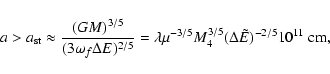
In this Paper we assume that there is a black hole of mass
 -
in a star
cluster and estimate the rate of capture
of white dwarfs of mass m by the black hole. The capture rate is always
determined by the interplay of two processes. These are
the effect of distant two body
gravitational encounters changing the orbital angular momenta of the
stars and an interaction associated with
the presence of the black hole
which removes the orbital energy of a star and is effective only
when the orbital angular momentum is sufficiently small.
This type of interaction
may result either through tidal interactions or by the emission
of gravitational waves induced by the stellar orbital motion.
-
in a star
cluster and estimate the rate of capture
of white dwarfs of mass m by the black hole. The capture rate is always
determined by the interplay of two processes. These are
the effect of distant two body
gravitational encounters changing the orbital angular momenta of the
stars and an interaction associated with
the presence of the black hole
which removes the orbital energy of a star and is effective only
when the orbital angular momentum is sufficiently small.
This type of interaction
may result either through tidal interactions or by the emission
of gravitational waves induced by the stellar orbital motion.
The efficiency of tidal interactions is determined by the ratio of orbital pericentre
distance to the tidal radius - the latter being the distance
from the black hole below which significant disruption of the star
through mass loss induced by tides occurs.
On the other hand, the efficiency of
orbital energy loss due to gravitational wave
emission
is determined by the ratio of the
orbital pericentre distance to the gravitational radius of the black hole.
Since the tidal radii corresponding to white dwarfs
for the range of black hole masses considered here
are larger than their gravitational radii,
orbital energy is
changed mainly through the action of dynamical tides.
This is in contrast to the case of the more
massive black holes residing in galactic centres where emission of
gravitational waves is
more effective for changing the orbital energy of
white dwarfs (e.g. Ivanov 2002; Freitag 2003, and references therein).
Since the relative contribution
of two body gravitational encounters to the orbital evolution
decreases very sharply for small angular momenta, a star with sufficiently
small angular momentum loses orbital energy through tidal interaction
while the orbital angular momentum remains approximately unchanged.
The latter occurs because the star cannot store a significant amount of angular
momentum in comparison to the orbit.
Accordingly, the orbital eccentricity decreases
during this process which will be referred to as
orbital circularisation.
As a result of this process a tight
quasi-circular orbit around a black hole may be formed. A white
dwarf on such an orbit can emit gravitational radiation in the
frequency band of order of 10-2 Hz which is the
most favoured for the planned LISA space borne gravitational wave
antenna. In principal this is able to detect gravitational waves
with dimensionless amplitude as small as 10-24, for an
observational time of one year. That means that the presence of such
a white dwarf
can be detected from distances of order of 103 Mpc.
Taking into account the fact that globular clusters form a very abundant
population of cosmic objects such systems may contribute significantly
to the budget of sources of gravitational radiation available for LISA.
There is one principal obstacle inhibiting formation of
a binary pair consisting of a black hole of mass M and a white
dwarf of mass m in a tight orbit around it. Because it is produced
through tidal interaction, its semi-major
axis will be close to the tidal radius. There the ratio of orbital binding
energy to gravitational energy of the white dwarf is of order
of
 .
Thus, for
such an orbit to be produced, an amount of energy far exceeding the internal binding energy of
the white dwarf must be removed from it. When tides are
effective, orbital energy is transferred to pulsation
modes and thence to the internal energy of the star.
Therefore, without an effective energy loss
mechanism, the white dwarf could be easily unbound and thus
destroyed by the tidal
input of energy or tidal inflation.
.
Thus, for
such an orbit to be produced, an amount of energy far exceeding the internal binding energy of
the white dwarf must be removed from it. When tides are
effective, orbital energy is transferred to pulsation
modes and thence to the internal energy of the star.
Therefore, without an effective energy loss
mechanism, the white dwarf could be easily unbound and thus
destroyed by the tidal
input of energy or tidal inflation.
Here we propose and discuss such a
mechanism, which may, in principle, allow unbinding due to tidal energy input to be circumvented for
a range of orbital parameters of the star. The operation of this mechanism
depends on the interplay of several factors influencing the orbital
evolution of star which we introduce below.
The character of orbital evolution under the influence
of tides is mainly determined by three factors: 1) the time scale for
decay of the stellar pulsations excited by tidal interaction, 2) the orbital
parameters of the star, and 3) the rotation of the star.
Let us first consider the decay of pulsations in
a non-rotating star. In this paper we assume that decay of
stellar pulsations is caused both by the emission of gravitational waves
that occurs because of the time-dependent
density perturbations associated with them,
and also by the dissipation of pulsation energy leading to its conversion
into internal energy of the star.
The latter decay channel is assumed to result through non-linear effects.
Since its properties are very poorly understood at the present time,
we shall consider the corresponding dissipation time scale to be a free
parameter. But we shall assume that it is larger
than the orbital period of the star. However, this is not an essential
assumption for orbital evolution at sufficiently large
semi-major axes, see below.
Initially the stellar orbit will be highly eccentric with a tidal interaction
that excites stellar pulsations occurring impulsively at pericentre passage (e.g. Lai 1997; Ivanov
Papaloizou 2004, hereafter IP). For long decay time scales,
pulsations will always be present in the star, and as a result of every periastron passage, a new perturbation excited by tides is added.
When orbital semi-major axis is sufficiently large or the orbital period sufficiently long,
it has been established that tidally induced changes to it cause the phase correlation between
preexisting pulsations and freshly excited ones to be lost.
Then, both the energy content of excited pulsation modes and the orbital energy of the
star evolve in a stochastic manner (e.g. Kochanek 1992; Kosovichev Novikov 1992; Mardling 1995). Under this evolution, the mode energy and the orbital
binding energy of the star grow on average, with a part of the mode
energy being transferred to the internal energy of the star. Therefore the
stochastic exchange of energy between the orbit and stellar pulsations leads to a decrease of the orbital semi-major axis and period as well as an increase of the internal energy of the star.
However, once the orbital period is sufficiently short,
or the semi-major axis is below a critical value,
pulsation modes can maintain phase coherence
between successive pericentre passages, stochastic evolution ceases
and dynamic tides are expected to become less efficient.
At this point, the tidal
evolution rate is determined by the natural decay timescales
of the pulsation modes. A steady pulsation energy
typical of that induced through one pericentre passage may be maintained, rather than the
growth that occurs through the cumulative effect
of mode energy inputs proceeding over many pericentre passages when the
semi-major axis is large.
An important issue is whether the internal energy added to the
star during the phase of stochastic evolution is enough to cause
its destruction.
For a non-rotating star the internal energy obtained by the star
when the critical semi-major axis is reached is larger than the stellar
gravitational energy. Therefore, such a star could be disrupted by tidal
heating before the critical semi-major axis is reached.
However, during orbital
circularisation orbital angular momentum is also transferred to the
star until an equilibrium rotation rate is attained.
This requires a rotation rate corresponding to
corotation at periastron or faster.
Thus the star can be spun up to high rotation
rates. When measured in terms of the amount of energy input per periastron passage,
the efficiency of tidal interaction is minimised for such a
rotating star. See for example Fig. 8 of Lai (1997) and also IP.
Accordingly the time scale of circularisation is increased.
In this situation, when dissipation of the mode energy
as a result of non linear effects is not effective,
the time scale for transmitting orbital
energy to the pulsation modes may be
larger than the time scale for removal
of the pulsation energy through gravitational
waves emitted because of the time-dependent perturbation of the star.
In this situation the white dwarf may reach the critical semi-major
axis without internal dissipation
causing tidal inflation
because of cooling by emission of gravitational waves.
In the opposite limit of effective mode dissipation and internal heating, the rapidly rotating
white dwarf may attain the critical semi-major axis
through the emission of gravitational waves induced by orbital motion
rather than through tidal interaction.
Thus taking into account the reduction
in effectiveness of the tidal
energy transfer brought about by the
effect of stellar rotation, we find that for sufficiently
large orbital angular momenta
the semi-major axis can be decreased
below the critical one without significant heating of the star.
After the critical semi-major axis is reached, again, because of the reduced
efficiency of the tidal interaction, orbital
evolution is governed by the emission of gravitational
waves determined by the orbital motion of the white
dwarf. This process can further reduce the orbital
semi-major axis and lead to formation of a tight
quasi-circular orbit.
We formulate the criterion for white dwarf "survival'' treating
dynamic tides within the framework of the simplest possible model
of tidal interactions. We assume that the internal structure
of a white dwarf is the same as that of a n=1.5 polytrope.
We also assume that the results obtained from the theory of dynamic
tides in slowly rotating stars can be extrapolated to
high rotation rates for the purpose of making
approximate estimates.
Based
on these assumptions we estimate the formation rate of tight
pairs which turns out to be an order of magnitude smaller than
the total rate of tidal capture, for typical parameters of the
problem. This allows us to obtain an estimate of
probability of detection of such sources of gravitational waves
by LISA. We conclude that LISA could, in principal, detect such
a source provided that there is a significant fraction of
globular clusters containing black holes with masses
103-
,
and with stellar velocity dispersions
in their innermost regions
exceeding 20 km s-1.
There are a number of different possibilities and branchings associated with the orbital evolution
subsequent to tidal capture. Each of these requires consideration of several physical
processes and is described by a number of algebraic expressions. In order to clarify
the situation, we provide a more transparent summary of the proposed paths to a circularised orbit with
disruption of the star avoided.
In Fig. 1
we give a diagrammatic illustration of the possible orbital evolutionary paths
that can be taken by
a white dwarf subsequent to tidal capture by an intermediate mass black hole.
Initially, impulsive energy and angular momentum exchanges between the
orbit and star that occur every pericentre passage spin it up and excite modes of oscillation.
As a result the rate of tidal evolution of the orbit decreases
such that gravitational radiation can become more
important. This may also be important for damping the oscillation modes.
If the tidal capture occurs at sufficiently large pericentre distance,
the importance of gravitational radiation during the orbital and pulsation mode evolution
may allow the star to survive the regime of impulsive energy input
at pericentre passage and become circularised without disruption and
be a potential LISA source.
![\begin{figure}
\par\includegraphics[width=8cm,clip]{7105fig1.eps}\end{figure}](/articles/aa/full/2007/46/aa7105-07/Timg26.gif) |
Figure 1:
A schematic illustration of the possible orbital evolutionary paths
of a white dwarf that is tidally captured by an intermediate mass black hole.
The star is initially scattered into a highly elongated trajectory that evolves
due to impulsive energy and angular momentum exchanges between the
star and orbit that occur every pericentre passage, the pericentre
distance remaining very nearly fixed. As a result of these,
the internal energy and angular momentum increase. However, this process is slowed
as the star spins up and under favourable conditions gravitational radiation can become
important so that it controls the orbital evolution and/or damps the excited pulsation modes.
The latter case a) leading to cases a1) and a2) occurs where other non linear processes are ineffective at dissipating the pulsations. Case b) leading to cases b1) and b2) occurs when such processes are more effective. For both cases a) and b) the star may survive the orbital evolution if the tidal capture occurs at sufficiently large pericentre distance. |
| Open with DEXTER |
The plan of the paper, in which the above phenomena are considered in
more detail, is as follows.
In Sect. 2 we describe the model of the stellar cluster
we use and the effect of distant two body encounters.
In Sect. 3 we go on to discuss the
tidal interaction of a white dwarf with the central black hole and
pulsation mode excitation through dynamic tides.
Then in Sect. 4 we consider the way in which
gravitational wave emission/non linear effects
may lead to pulsation mode amplitude limitation.
In Sect. 5 we go on to explore the
conditions for safe circularisation or tidal disruption of the white dwarf.
In Sect. 6 we discuss the rate of tidal capture of white dwarfs by the black hole
and estimate the fraction that can circularise safely, with technical
details being relegated to an Appendix.
In Sect. 7 we estimate the probability of detection of this source of gravitational
radiation. Finally in Sect. 8 we discuss our results.
2 The stellar system
In order to discuss the rate of orbital circularisation for
white dwarfs it is first
necessary to consider
the properties of the star cluster in which they
are situated. This is because dynamical interaction with the stars
in the system is responsible for the production
of orbits for which tidal interaction with the central black
hole becomes significant.
The radius of influence of the central
black hole, ra, is defined as the radius
within which the total mass of the stars is
the same as the mass of the central black hole:
 .
As has been noted by many authors, when
r < ra, a "cusp''
in the stellar distribution of stars is formed with a density distribution
such that
.
As has been noted by many authors, when
r < ra, a "cusp''
in the stellar distribution of stars is formed with a density distribution
such that
 |
(1) |
where the parameter p is typically small.
Two values that have been suggested through theoretical
considerations are p=0
(Young 1980) and p=1/4 (Gurevich 1964; Bahcall
Wolf 1976). Recently simulations by Baumgardt et al. (2004a,b) have indicated that for the case of globular clusters having a stellar population with a single mass,
 while for systems with a realistic multi-mass stellar population,
 ,
with
,
with
 for the most massive
stars.
for the most massive
stars.
In this paper we make only approximate estimates of the
tidal circularisation rate. Thus
for simplicity, we have adopted
p=0 for all components of the stellar system.
We note that if a steeper cusp profile were to be adopted,
the number of tidally captured stars at any particular time would increase by a
numerical factor of order unity.
Making the usual assumption that the phase space distribution function for
"typical'' stars depends on the binding energy per unit mass only
and the distribution of white dwarfs is the same as
that of typical stars, it can be easily shown from (1) with p=0that the distribution function for the white dwarfs
over binding energy per unit mass and specific angular momentum,
 ,
is
,
is
 |
(2) |
where M and m are the masses of the black hole and of a
typical star, and we assume that
 .
.
 is the number fraction of white
dwarfs in the cusp, E and J are, respectively,
the binding energy per unit mass and the
specific angular momentum of a star. We adopt the convention that the
binding energy has positive values for the gravitationally bound stars
considered in this paper.
is the number fraction of white
dwarfs in the cusp, E and J are, respectively,
the binding energy per unit mass and the
specific angular momentum of a star. We adopt the convention that the
binding energy has positive values for the gravitationally bound stars
considered in this paper.
 |
(3) |
is the orbital period of a star with binding energy per unit mass E.
The assumption of isotropy of the phase space distribution function
is applicable only for estimates of quantities
determined by the bulk of the stars, such as e.g. quantities
characterising distant gravitational interactions, see Eq. (5) below.
It becomes invalid
for stars with sufficiently low orbital angular momentum which
can either be tidally disrupted or
directly captured by the black hole.
The presence of the
black hole thus leads to the formation of a "loss cone''
such that Eq. (2)
over-estimates the number of stars having low angular momenta.
Assuming that stars with sufficiently
small specific angular momenta
 are absent,
the presence of the loss cone may be easily
accounted for by a correction factor (e.g. Lightman
Shapiro 1977)
such that the distribution function of the white dwarfs is modified to become
are absent,
the presence of the loss cone may be easily
accounted for by a correction factor (e.g. Lightman
Shapiro 1977)
such that the distribution function of the white dwarfs is modified to become
 |
(4) |
where
 ,
,
 ,
and
,
and
 is the specific angular momentum corresponding to a circular
orbit with a given value of the binding energy per unit mass E.
Typically,
is the specific angular momentum corresponding to a circular
orbit with a given value of the binding energy per unit mass E.
Typically,
 .
.
A star orbiting around the black hole changes its energy and
angular momentum due to distant gravitational interactions with
other stars in the cusp. These result in a random walk
in phase space. The stochastic change of the specific angular
momentum per orbital period may be characterised by its
dispersion,
 ,
which can be written in the form (e.g.,
Ivanov 2002):
,
which can be written in the form (e.g.,
Ivanov 2002):
 |
(5) |
where q=m/M is the mass ratio,
 and we use the dimensionless energy variable
  defined through
 .
.![[*]](/icons/foot_motif.gif)
3 Tidal interaction of a white dwarf with the central black hole
In order to make order of magnitude estimates
we use the simplest possible model for the
white dwarf. We assume zero temperature so that
the pressure is due to completely degenerate electrons.
In this case the equation of state is
baratropic and gravity or g modes are absent.
Furthermore we approximate the structure of the white dwarf as
that of a n=1.5 polytrope. In addition to the mass m and radius
 we introduce the two parameters
 and
and
 cm). The effectiveness of tidal interactions
depends significantly on the mean density of the white dwarf.
To characterise low and high density cases we consider two
sets of values for
cm). The effectiveness of tidal interactions
depends significantly on the mean density of the white dwarf.
To characterise low and high density cases we consider two
sets of values for  and
and  The "low density'' case will be characterised by parameters appropriate for
a "typical'' white dwarf for which
The "low density'' case will be characterised by parameters appropriate for
a "typical'' white dwarf for which  and
and
 ,
and
for the "high density'' case we use parameters corresponding
to Sirius B for which
,
and
for the "high density'' case we use parameters corresponding
to Sirius B for which
 and
and
 .
.
For a baratropic star only fundamental (f), pressure (p) and inertial modes can be excited by
tidal interaction. Since p-modes have large eigen-frequencies and inertial
modes are significant only for rather large orbital angular momenta
(Papaloizou
Ivanov 2005),
their respective contributions to the tidal exchange of energy and
angular momentum are small compared to the contribution of the
f-modes for the range of the orbital parameters of
interest, so they are not considered further.
To make our estimates, we use the linear theory of tidal
perturbations induced in a slowly rotating star and consider
only the leading order quadrupole response. The assumption
of slow rotation is certainly valid in the early
stages of orbital evolution due to tides. In this regime orbital changes
induced by distant gravitational interactions and tidal effects compete
with each other. Then we may assume that the star is non-rotating
when calculating the rate of tidal circularisation.
However, the
star can be spun up because of the effect of tides during
orbital circularisation,
achieving a considerable rotation rate during the later stages.
As we will see below this may have important
implications for the outcome of the orbital evolution of the star.
In particular, it may play a role in determining
whether is it possible or not for the star to survive in
a tight quasi-circular orbit. Therefore,
it is directly related to the problem of formation of sources
of gravitational radiation. Unfortunately, a theory of tidal
perturbations of a fast rotating star is practically undeveloped
in the present time. Accordingly, we shall assume that the
results obtained from the theory of slowly rotating stars can
be extrapolated to the case of fast rotation for the purposes of making
order of magnitude estimates.
During the early stages of tidal circularisation, the orbit of the star
is highly eccentric. In this case tidal
interactions are only important near pericentre. Because of this, in order to
calculate the energy and angular
momentum exchange between the orbit and the modes of pulsation of
the star
it is possible to consider it as undergoing a sequence of successive
flybys of the black hole each of which produces an impulsive change.
This formulation of the problem allows us to use
the theory of tidal excitation and dissipation of
the fundamental modes in a baratropic star moving on a highly
eccentric or parabolic orbit developed elsewhere
(see e.g. Press & Teukolsky 1977, hereafter PT;
Lai 1997, IP).
This theory is based on consideration
of a single pericentre passage where an amount of energy
 and an amount of angular
momentum
and an amount of angular
momentum  is transferred from the orbit to the star.
These quantities depend on the amplitudes and phases of the pulsation modes
before the passage and on the radius of pericentre,
is transferred from the orbit to the star.
These quantities depend on the amplitudes and phases of the pulsation modes
before the passage and on the radius of pericentre,  .
.
Let us temporarily assume that the amplitude of the pulsation mode
before pericentre passage is negligible and the stellar model
and the angular velocity of the star are fixed. In this case, it can be shown that the quantities
and
are determined by the value of dimensionless parameter (PT)
 |
(6) |
where
is the pericentre distance. These quantities can
be naturally considered as being made up of two parts: 1) a quasi-static part
determined by irreversible loss of total energy of the system during the pericentre passage and 2) a dynamic part (due to the so-called dynamic tide) determined by excitation
of the normal modes of the star.
The quasi-static part of the energy transfer
 ,
can be written in the form:
,
can be written in the form:
 ,
where
,
where
 is some "reference''
energy associated with the star and the dimensionless coefficient
is some "reference''
energy associated with the star and the dimensionless coefficient
 is determined by the dissipative processes operating in the star. An explicit expression for
can be found in IP. During the flyby
energy loss occurs as a result of
viscous dissipation in the bulk of
the white dwarf and in its convective envelope and also
due to emission of gravitational waves. Since the coefficient
of dynamic viscosity in the bulk of the white dwarf appears
to be very small (104-106 in cgs units, e.g. Chugunov
Yakovlev 2005, and references therein) and convective
envelopes of white dwarfs also have a rather small estimated
turbulent viscosity and a very small relative mass, their
respective contributions to the coefficient
are
quite small. The main contribution appears to come from
the emission of gravitational waves generated by time dependent
perturbation of the white dwarf (see Osaki
Hansen 1973, hereafter OH). However, a simple estimate shows that the value of
determined by this process
leads to a value of
much smaller than
that associated with dynamic tides, for relevant values
of
is determined by the dissipative processes operating in the star. An explicit expression for
can be found in IP. During the flyby
energy loss occurs as a result of
viscous dissipation in the bulk of
the white dwarf and in its convective envelope and also
due to emission of gravitational waves. Since the coefficient
of dynamic viscosity in the bulk of the white dwarf appears
to be very small (104-106 in cgs units, e.g. Chugunov
Yakovlev 2005, and references therein) and convective
envelopes of white dwarfs also have a rather small estimated
turbulent viscosity and a very small relative mass, their
respective contributions to the coefficient
are
quite small. The main contribution appears to come from
the emission of gravitational waves generated by time dependent
perturbation of the white dwarf (see Osaki
Hansen 1973, hereafter OH). However, a simple estimate shows that the value of
determined by this process
leads to a value of
much smaller than
that associated with dynamic tides, for relevant values
of  .
Therefore, the overall contribution of quasi-static tides appears to be negligible
and will not be considered further.
.
Therefore, the overall contribution of quasi-static tides appears to be negligible
and will not be considered further.
Now let us consider dynamic tides associated with
the fundamental quadrupole mode of pulsation. As was shown by IP
for the case of a slowly rotating star,
the quadrupole mode propagating in the direction of orbital motion
(the so-called prograde mode) determines the exchange
of energy between the orbit and the star provided that
the angular frequency of the star,
 ,
is
smaller that its "equilibrium'' value
,
is
smaller that its "equilibrium'' value
 ,
where
,
where
 is a "reference''
frequency associated with the star. As it
will be shown later, in our problem a typical value
of
is a "reference''
frequency associated with the star. As it
will be shown later, in our problem a typical value
of
 ,
and the equilibrium angular frequency
,
and the equilibrium angular frequency
 is formally larger than
the angular frequency at rotational break-up of the star,
is formally larger than
the angular frequency at rotational break-up of the star,
 .
Although the theory
leading to this conclusion is not valid at such high rotation
rates, it seems reasonable to assume that the energy exchange
is mainly determined by the prograde mode unless a rate of
rotation very close to
.
Although the theory
leading to this conclusion is not valid at such high rotation
rates, it seems reasonable to assume that the energy exchange
is mainly determined by the prograde mode unless a rate of
rotation very close to
 is reached.
Considering excitation of only this
mode and assuming that the star is not
perturbed before pericentre passage, it easy to see
from results given in IP that the energy gained by the
star per unit of mass,
is reached.
Considering excitation of only this
mode and assuming that the star is not
perturbed before pericentre passage, it easy to see
from results given in IP that the energy gained by the
star per unit of mass,
 can be expressed as
 |
(7) |
where we use the fact that the eigenfrequency
of the quadrupole f mode for a non-rotating n=1.5 polytrope
 and the value of dimensionless "overlap'' integral
 calculated in, e.g., Lee & Ostriker (1986). The quantity
 characterises the
strength of the tidal interaction for a non-rotating star
and
characterises the
strength of the tidal interaction for a non-rotating star
and  determines correction to the energy exchange due to
rotation, being unity for a non rotating star (see below).
Explicitly, we have
determines correction to the energy exchange due to
rotation, being unity for a non rotating star (see below).
Explicitly, we have
 |
(8) |
where
is given by Eq. (6). When
 -2, the
white dwarf is either tidally disrupted or stripped, and
the linear theory of dynamic tides cannot be used (see e.g. Frolov et al. 1994; Ivanov
Novikov 2001, and references therein). As it will be shown later, typically,
-5 for white dwarfs undergoing tidal circularisation.
Since the energy gain decreases exponentially with
the use
of the linear theory seems to be justified in our case.
-2, the
white dwarf is either tidally disrupted or stripped, and
the linear theory of dynamic tides cannot be used (see e.g. Frolov et al. 1994; Ivanov
Novikov 2001, and references therein). As it will be shown later, typically,
-5 for white dwarfs undergoing tidal circularisation.
Since the energy gain decreases exponentially with
the use
of the linear theory seems to be justified in our case.
The characteristic pericentre distance below which tidal disruption is expected
is determined as the distance where the tidal force acting on an element of the star near its surface is comparable to the gravitational force due to the star itself. Thus it is given by
 |
(9) |
where
 .
Using this
we can rewrite Eq. (6) in another form
.
Using this
we can rewrite Eq. (6) in another form
 |
(10) |
where
 is the specific orbital angular momentum of an orbit with pericentre distance equal to rT. From Eq. (10) it follows that when

 is also approximately conserved.
The black hole mainly tidally disrupts the white dwarfs
provided that its mass is sufficiently small.
To see this we note that the specific orbital angular
momentum of stars directly captured by the black hole must be smaller
than
 .
Define the "critical'' mass
.
Define the "critical'' mass
 by the condition
that
by the condition
that
 when
when
 One obtains
 |
(11) |
When
 ,
the specific angular momentum JT exceeds
,
the specific angular momentum JT exceeds
 so it
determines the boundary of the loss cone. Thus
so it
determines the boundary of the loss cone. Thus
 and, accordingly,
 (recall that
  is defined as
).
is defined as
).
As indicated above, the rotation rate of the star has an
important effect in determining the strength of the tidal interaction.
From the results given in IP it follows that the corresponding
correction factor
entering in Eq. (7) has the form
 |
(12) |
where
 ,
,
 is the angular velocity of the star and we recall that
 characterises a typical
frequency of stellar pulsation associated with the fundamental
mode. It is important to note that Eq. (12) has been formally
derived assuming that
characterises a typical
frequency of stellar pulsation associated with the fundamental
mode. It is important to note that Eq. (12) has been formally
derived assuming that
 .
However, we are going to use it later on to make our
estimates implying that it is approximately valid when
.
However, we are going to use it later on to make our
estimates implying that it is approximately valid when
 .
Note that this assumption may be justified in part by results of
calculations of Managan (1986) who considered normal modes of
a fast rotating n=1.5 polytrope and
of Clement (1989) who considered those of a fast rotating
15
.
Note that this assumption may be justified in part by results of
calculations of Managan (1986) who considered normal modes of
a fast rotating n=1.5 polytrope and
of Clement (1989) who considered those of a fast rotating
15  star. In both cases it was
found that the eigen frequency of the
prograde f mode has an approximate linear dependence
on the frequency of rotation until an angular frequency very
close to
is reached. The linear dependence
of the eigen frequency on the frequency of rotation appears to
be one of the most important factors leading to Eq. (12).
star. In both cases it was
found that the eigen frequency of the
prograde f mode has an approximate linear dependence
on the frequency of rotation until an angular frequency very
close to
is reached. The linear dependence
of the eigen frequency on the frequency of rotation appears to
be one of the most important factors leading to Eq. (12).
3.7 The effect of many pericentre passages and the criterion for
stochastic instability
Let us consider a sequence of many pericentre flybys assuming that
the energy per unit mass contained in modes of oscillation, Em, does not
decay significantly between successive pericentre passages. In this
case there is interference between the preexisting wave perturbation
in the star and the wave excited in the vicinity of pericentre as a
result of tidal perturbation. In this case, simple addition of (7) to Em after the pericentre passage to obtain
the new Em needs further justification. In this context it is important that the
orbital period
 is changing with time as a result of tidal
interaction and loss of orbital energy due to emission of
gravitational waves, and therefore
the the phase change of the oscillating mode generated
between two successive pericentre passages,
is changing with time as a result of tidal
interaction and loss of orbital energy due to emission of
gravitational waves, and therefore
the the phase change of the oscillating mode generated
between two successive pericentre passages,
 ,
is also changing with time.
When the change of
,
is also changing with time.
When the change of  during one orbital period,
 is larger than
  ,
the mode phase at the time of the next pericentre passage is essentially a random quantity, and accordingly, the mode
energy per unit mass
,
the mode phase at the time of the next pericentre passage is essentially a random quantity, and accordingly, the mode
energy per unit mass  evolves as a stochastic variable. In this case
we can add expression (7) to
at each pericentre passage on average,
assuming that all resulting expressions are valid in some statistical
sense being averaged over many realisations of the stochastic
process. The process of stochastic evolution of the mode
energy will be refereed to as "stochastic instability''.
evolves as a stochastic variable. In this case
we can add expression (7) to
at each pericentre passage on average,
assuming that all resulting expressions are valid in some statistical
sense being averaged over many realisations of the stochastic
process. The process of stochastic evolution of the mode
energy will be refereed to as "stochastic instability''.
A condition for the stochastic instability to operate can be
readily found from the condition
 and the expression (3) for the orbital period in the form
 |
(13) |
where a is the orbit semi-major axis,
 |
(14) |
is the dimensionless change of the orbital energy per unit mass,  in one
orbital period, and
in one
orbital period, and
 is the change of the orbital
energy per unit of mass during one orbital period
due to emission of gravitational waves, see Eq. (28) below
for an explicit expression. As follows from Eq. (14) the condition for the stochastic instability to set in involves two contributions to the change of the orbital energy:
associated with tides and
determined by gravitational waves emitted as a result of orbital
motion. This differs from the case of tidally interacting
stellar binaries where only the tidal contribution is normally
considered. In the case of stellar binaries, when the stochastic
instability operates, both the orbital binding energy and the energy
of the mode of pulsation evolve in a stochastic manner (e.g. Mardling
1995). The fact that
enters into Eq. (14) leads to the possibility of the stochastic instability operating in a situation where orbital evolution is mainly
determined by emission of gravitational waves, i.e.
is the change of the orbital
energy per unit of mass during one orbital period
due to emission of gravitational waves, see Eq. (28) below
for an explicit expression. As follows from Eq. (14) the condition for the stochastic instability to set in involves two contributions to the change of the orbital energy:
associated with tides and
determined by gravitational waves emitted as a result of orbital
motion. This differs from the case of tidally interacting
stellar binaries where only the tidal contribution is normally
considered. In the case of stellar binaries, when the stochastic
instability operates, both the orbital binding energy and the energy
of the mode of pulsation evolve in a stochastic manner (e.g. Mardling
1995). The fact that
enters into Eq. (14) leads to the possibility of the stochastic instability operating in a situation where orbital evolution is mainly
determined by emission of gravitational waves, i.e.
 ,
see Sect. 5 and the Appendix. In this limit, our numerical investigations indicate that the orbital binding energy can increase in a way that appears to be fairly regular while the energy of the pulsation mode still tends to increase in an erratic manner. On the other hand, the mode energy ceases to increase when
,
see Sect. 5 and the Appendix. In this limit, our numerical investigations indicate that the orbital binding energy can increase in a way that appears to be fairly regular while the energy of the pulsation mode still tends to increase in an erratic manner. On the other hand, the mode energy ceases to increase when
 and
and
 0.05. We have checked that the condition
0.05 is fulfilled for parameters typical for our problem.
0.05. We have checked that the condition
0.05 is fulfilled for parameters typical for our problem.
It is interesting to note that the condition (13) can be also derived from quite
a different approach based on the treatment of the tidal interaction
as occurring through resonances between the mode frequency
 and the changing orbital frequency
 of different
order n, such that
of different
order n, such that
 .
The
condition of overlap of these resonances given that
is changing is
.
The
condition of overlap of these resonances given that
is changing is
 This is equivalent to the condition (13).
4 Gravitational wave emission/non-linear effects, characteristic time scales
and mode amplitude limitation
As we have mentioned above the most important linear decay channel of
the fundamental mode appears to be through emission of
gravitational waves. The corresponding decay time of the fundamental
mode has been calculated by OH for two models of iron
white dwarfs. The results can be extended to the range of
masses and radii appropriate for "standard'' CO white
dwarfs with help of the expression for the gravitational
wave luminosity, LGW, produced by the oscillating mode and the resulting decay time
can be expressed as
 |
(15) |
Note we define the decay time as
 which gives a value of
 which is a factor of two smaller compared
to that of OH.
which is a factor of two smaller compared
to that of OH.
In this situation the mode energy can attain a large value
as a result of the cumulative effect of
multiple tidal interactions occurring at pericentre passage.
At high amplitudes non linear effects may lead to additional
dissipation and mode decay.
We characterise such effects by adopting a mode decay time scale
tnl which is a function of the mode
energy. The non linear theory for these pulsation modes
is not yet adequately developed to provide a form for tnl. Therefore,
we regard this as a free parameter and consider
two limiting cases: a) the time tnl is assumed to be large
compared to
,
being taken to be
comparable to
 ,
the actual time scale of orbital evolution
which is the smaller of the times required to change the
orbit significantly through tidal interaction or to make it evolve as
a result of the emission of gravitational waves induced
by that orbital motion, see below Eq. (22).
Assuming that all quantities characterising the mode of pulsation and the star
evolve on the time scale of order of
,
we estimate below that the condition
,
the actual time scale of orbital evolution
which is the smaller of the times required to change the
orbit significantly through tidal interaction or to make it evolve as
a result of the emission of gravitational waves induced
by that orbital motion, see below Eq. (22).
Assuming that all quantities characterising the mode of pulsation and the star
evolve on the time scale of order of
,
we estimate below that the condition
 is equivalent to the condition that the rotational angular momentum
of the star is the same order of magnitude as the angular momentum corresponding to the
mode, see Eq. (18) below. Thus, in this situation the degree of non-linearity
adjusts in a way that does not allow the mode angular momentum to significantly exceed that in
the stellar rotation.
b) The time
is equivalent to the condition that the rotational angular momentum
of the star is the same order of magnitude as the angular momentum corresponding to the
mode, see Eq. (18) below. Thus, in this situation the degree of non-linearity
adjusts in a way that does not allow the mode angular momentum to significantly exceed that in
the stellar rotation.
b) The time
 is assumed to be short compared to both
and
the orbital evolution time scale
is assumed to be short compared to both
and
the orbital evolution time scale
 However, in both cases we shall assume that tnl
is much larger than the orbital period of the tidally interacting star.
But note that this is not strictly necessary during the first phase of evolution
when the semi-major axis is large (see Sect. 4.1 below)
However, in both cases we shall assume that tnl
is much larger than the orbital period of the tidally interacting star.
But note that this is not strictly necessary during the first phase of evolution
when the semi-major axis is large (see Sect. 4.1 below)
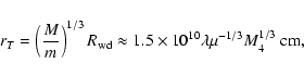
4.1 Balance of mode energy and angular momentum
input due to tides and losses due to
gravitational radiation/non linear effects
Here we estimate the amount of mode energy
that is stored in the star when there is a balance between
the build-up of mode energy due to
the stochastic instability and decay due to the emission of gravitational
waves or non linear effects.
Provided this balance can occur with a stellar
mode angular momentum content that is small enough to avoid break up
of the star,
it is possible for it to
avoid disruption by having to absorb a large amount
of released orbital binding energy.
In a stationary state
the mode energy per unit of mass can be estimated from the balance equation
 |
(16) |
The mode specific angular momentum, Lm, is related to Em by the
standard equation:
 |
(17) |
where we take into account that tides mainly excite the quadrupole mode
with the azimuthal mode number m=2.
The rate of transfer of angular momentum to the star is
related to the rate of dissipation of mode energy
(e.g. Goldreich & Nicholson 1989) and thus determined by
tnl. The rate of transfer of specific angular momentum is
 and accordingly the
total specific angular momentum transferred to the star in a time
interval
is estimated to be
and accordingly the
total specific angular momentum transferred to the star in a time
interval
is estimated to be
 |
(18) |
Obviously, L* should not exceed the specific angular momentum of
the star in a state of uniform rotation with angular frequency
corresponding to rotational break-up.
Estimating the moment of
inertia of the star per unit of mass as
 and
using the standard relation
and
using the standard relation
 ,
from Eqs. (16)-(18) we obtain
the associated dimensionless angular velocity of the star
to be given by
,
from Eqs. (16)-(18) we obtain
the associated dimensionless angular velocity of the star
to be given by
 |
(19) |
where we introduce the characteristic time
for tidal build-up of the mode energy
 |
(20) |
Note that tT so defined can formally be smaller than
.
It is obvious that in that case it is the orbital period
which plays the role of the characteristic tidal time scale.
Substituting Eq. (7) in (20) we can express the tidal time scale in the form
 |
(21) |
where
r1=ra/(1 pc). Note that since
 typically we have
 yr.
yr.
In general the time scale of orbital evolution
is given by
 |
(22) |
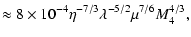
where tGW is the characteristic time of orbital evolution
due to gravitational wave emission explicitly given below,
see Eq. (29).
As indicated below, for a white dwarf
spun up through tidal interaction, gravitational
waves emitted as a consequence of orbital motion
are more effective than tides at
inducing orbital evolution. In this case

Recalling that the break up angular velocity
,
and assuming that
the criterion
 provides the condition for the
white dwarf to survive the circularisation process,
we obtain a limitation on the orbital binding energy per unit mass
of the white dwarf, during the phase of stochastic instability,
to be given by
provides the condition for the
white dwarf to survive the circularisation process,
we obtain a limitation on the orbital binding energy per unit mass
of the white dwarf, during the phase of stochastic instability,
to be given by
 |
(23) |
This equation leads to
a constraint that the orbital binding energy of the white dwarf should
not be too high while mode energy input as implied by the existence of
stochastic instability is occurring. The condition (23) can be simplified
when tnl is either large or small. For case a) when
 the condition (23) can be written as
 |
(24) |
where we recall that the dimensionless energy
is related
to the orbital binding energy per unit mass E as
 .
This condition can be reformulated as setting
an upper bound on the allowed mode energy per unit mass as
.
This condition can be reformulated as setting
an upper bound on the allowed mode energy per unit mass as
 |
(25) |
Note that in case a) the angular momentum transferred to stellar rotation
is approximately equal to that associated with the mode of pulsation.
Therefore the condition
can be regarded
as a condition for equipartition of the angular momentum associated with the pulsation
mode and that associated with the stellar rotation.
In the opposite limit corresponding to case b) we have
 Then Eq. (23) gives
 |
(26) |
In this case the energy put into internal energy of the star,
 ,
through dissipation
is much larger than the mode energy, Em, and we can express (26) as leading to an upper bound for
in a form analogous to that given by (25)
,
through dissipation
is much larger than the mode energy, Em, and we can express (26) as leading to an upper bound for
in a form analogous to that given by (25)
 |
(27) |
We remark that this condition, obtained from considerations
of the stellar rotation, is equivalent to specifying a limit
on the allowed increase of the internal energy.
As almost all of the orbital binding energy is
converted to internal energy of the star in case b),
the same constraint would occur if the initial evolutionary phase involving stochastic instability
were replaced by one in which the energy input into oscillations during each pericentre passage was dissipated before the next one. Thus, as indicated in Sect. 4 above, the condition that
tnl should be less than the orbital period is not strictly necessary
during the initial evolutionary phase following tidal capture
(see also IP).
Note too that we have neglected the change of
the white dwarf radius due to tidal
heating. Assuming this change is modest, we can take it into account
by considering the white dwarf to have a slightly smaller mean density
when discussing conditions for safe circularisation, see
the next section.
4.2 Effect of gravitational radiation on the orbit
The change of orbital energy per unit mass
due to emission of gravitational waves generated by orbital motion
of the star can be obtained from results given by
Peters (1964). In the case of a highly eccentric orbit,
the change per orbital period, which is mainly induced at pericentre
may be written in the form
 |
|
|
|
 |
|
|
(28) |
and the corresponding evolution time can be expressed in terms
of tT as
 |
(29) |
Since the corresponding quantity induced by
tides,
,
decreases with
exponentially and
as an inverse power of ,
there is
a certain value of
where
tT=tGW. At larger
values of
the orbital evolution is mainly determined
by emission of gravitational waves. For non rotating stars (i.e. setting  )
this value of
is approximately equal to 5.3 for a "high density'' white
dwarf and 5.6 for a "low density'' white dwarf. As we have mentioned above and will discuss below, a typical value of
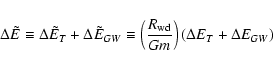
for the stars undergoing tidal circularisation is of the order of 4 and always smaller than 5. Taking into account that tT increases very rapidly with this parameter, we can conclude that tidal
interactions play the most significant role in the formation of a
flow of stars undergoing orbital circularisation.
)
this value of
is approximately equal to 5.3 for a "high density'' white
dwarf and 5.6 for a "low density'' white dwarf. As we have mentioned above and will discuss below, a typical value of
for the stars undergoing tidal circularisation is of the order of 4 and always smaller than 5. Taking into account that tT increases very rapidly with this parameter, we can conclude that tidal
interactions play the most significant role in the formation of a
flow of stars undergoing orbital circularisation.
On the other hand, the star is spun up by tides during
ongoing orbital circularisation and
tT is increased as a result. Therefore, at a later stage,
the orbital evolution may be governed by emission of
gravitational waves when the orbital binding energy is sufficiently
large, depending on parameters of the white dwarf
and of the star cluster.
Moreover, when the binding energy exceeds the value corresponding
to the onset of stochastic instability, the tidal response
becomes quasi periodic and
ineffective so that the orbital evolution is solely determined by the
emission of gravitational waves.
5 Conditions for safe circularisation or tidal disruption
Before going on to estimate of the rate of tidal capture and
circularisation we use the results of the previous
sections to examine more closely the conditions
required for mode amplitude limitation due to gravitational wave emission
to enable safe circularisation with the possibility of tidal
heating, inflation and disruption avoided.
During the early evolutionary phases,
subsequent to tidal capture, the star's orbit is highly eccentric, and the orbital
angular momentum is approximately conserved during the orbital
evolution while the semi-major axis/binding energy as well
as the angular velocity of the star change with time (see e.g. IP).
When tides dominate over the emission of gravitational waves induced by orbital motion, the
evolution time scale of the semi-major axis is given by
Eq. (20) and we have
 .
When gravitational radiation
controls the orbital evolution, which happens at large enough orbital binding energy,
we have
.
When gravitational radiation
controls the orbital evolution, which happens at large enough orbital binding energy,
we have
 where tGW is given by Eq. (29). For a given value of the orbital angular momentum, the orbital evolution time
depends on the orbital energy
E, and thus, on the star's semi-major axis a. This dependence
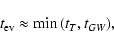
can be found from Eqs. (19)-(25) and (29). For illustrative purposes we plot this dependence as well as that of other characteristic time-scales in
Figs. 1 and 2 for a "low density'' white dwarf orbiting around a
black hole.
The cusp size is taken to be 1 pc. All dependencies are calculated in assumption that the stochastic instability operates for the shown range of binding energies.
where tGW is given by Eq. (29). For a given value of the orbital angular momentum, the orbital evolution time
depends on the orbital energy
E, and thus, on the star's semi-major axis a. This dependence
can be found from Eqs. (19)-(25) and (29). For illustrative purposes we plot this dependence as well as that of other characteristic time-scales in
Figs. 1 and 2 for a "low density'' white dwarf orbiting around a
black hole.
The cusp size is taken to be 1 pc. All dependencies are calculated in assumption that the stochastic instability operates for the shown range of binding energies.
![\begin{figure}
\par\includegraphics[width=8cm,clip]{7105fig2.eps}\end{figure}](/articles/aa/full/2007/46/aa7105-07/Timg153.gif) |
Figure 2:
Characteristic time scales in
years as functions of the dimensionless orbital energy  Plotted here are
,
the decay time of the
pulsation mode due to emission of gravitational waves associated with
the stellar pulsation,
,
the time scale for evolution of the orbit, tT, the
time scale of build-up of the mode energy and Plotted here are
,
the decay time of the
pulsation mode due to emission of gravitational waves associated with
the stellar pulsation,
,
the time scale for evolution of the orbit, tT, the
time scale of build-up of the mode energy and
 ,
the time scale of orbital evolution due to emission of gravitational waves induced by orbital motion. The horizontal dotted line 1 represents
.
The two solid curves 2a and 2b represent
calculated assuming that the stellar rotation frequency is given by Eq. (19).
The curve 2a taking on larger values at small values of
represents the case
,
and the other curve represents the case ,
the time scale of orbital evolution due to emission of gravitational waves induced by orbital motion. The horizontal dotted line 1 represents
.
The two solid curves 2a and 2b represent
calculated assuming that the stellar rotation frequency is given by Eq. (19).
The curve 2a taking on larger values at small values of
represents the case
,
and the other curve represents the case
 .
The inclined dotted line 3 represents tGW which becomes equal to
at the larger binding energies where gravitational radiation controls the orbital evolution. The dashed and dot dashed lines 4 and 5 represent tT calculated for .
The inclined dotted line 3 represents tGW which becomes equal to
at the larger binding energies where gravitational radiation controls the orbital evolution. The dashed and dot dashed lines 4 and 5 represent tT calculated for
 and
and
 ,
respectively. The dot dot dashed curves 6a and 6b represent tT calculated for the star rotating with angular frequency
given by Eq. (19) for values of binding energies larger
than that corresponding to the intersection of
and
.
For
smaller values of energies we have ,
respectively. The dot dot dashed curves 6a and 6b represent tT calculated for the star rotating with angular frequency
given by Eq. (19) for values of binding energies larger
than that corresponding to the intersection of
and
.
For
smaller values of energies we have
 .
Note the slower evolution due to tides
for the faster rotation rate. This results in gravitational radiation ultimately controlling the orbital evolution. All curves are calculated for ,
, .
Note the slower evolution due to tides
for the faster rotation rate. This results in gravitational radiation ultimately controlling the orbital evolution. All curves are calculated for ,
,
 ,
r1=1 and M4=1. ,
r1=1 and M4=1. |
| Open with DEXTER |
In Fig. 1 the characteristic time-scales corresponding
to a star with
are shown. The horizontal line indicates the
decay time scale of the stellar pulsations due to the emission of gravitational waves,
,
given by Eq. (15). The inclined dotted line indicates the dependence
of the characteristic time tGW on
and the inclined dashed and dot-dashed lines
show the dependence of tT on
for
 (dashed line) and
(dot-dashed line). We recall that the timescale tT applies to the
evolutionary phase just after tidal capture which can exhibit stochastic instability.
It may not be applicable to the later stages, when
is large, and
the conditions for additive impulsive energy inputs at pericentre passage
are not satisfied, see discussion below.
(dashed line) and
(dot-dashed line). We recall that the timescale tT applies to the
evolutionary phase just after tidal capture which can exhibit stochastic instability.
It may not be applicable to the later stages, when
is large, and
the conditions for additive impulsive energy inputs at pericentre passage
are not satisfied, see discussion below.
For a given value of ,
the dot-dashed line corresponding to a non rotating star, gives the smallest possible
value of
 .
For fixed ,
stars with
values tT exceeding that given by the dashed line, would have angular
velocities exceeding
,
and so would be disrupted.
Therefore the dashed curve gives the largest allowed value of
.
For fixed ,
stars with
values tT exceeding that given by the dashed line, would have angular
velocities exceeding
,
and so would be disrupted.
Therefore the dashed curve gives the largest allowed value of
 .
.
The solid curves indicate the evolution of
with
which is given by Eq. (19). The two different curves
correspond to the different assumptions about the value of the mode decay time due to
non-linear effects, tnl. The curve which is uppermost
at small values of
corresponds to the case a) where we assume that
while the other solid curve corresponds to the case b)
for which tnl is much less than both
and
.
One can see from Figs. 2 and 3 that the behaviour of the
characteristic time-scales is rather similar for these two cases. When
is very small, rotation of the star is small, and both curves are close to the dot-dashed line. Also, for small
values of
we have
.
![\begin{figure}
\par\includegraphics[width=8cm,clip]{7105fig3.eps}\end{figure}](/articles/aa/full/2007/46/aa7105-07/Timg157.gif) |
Figure 3:
Same as Fig. 1 but for  .
Note that in this case we have .
Note that in this case we have
 for the whole range of binding energies shown.
 |
| Open with DEXTER |
When
increases, the star
is spun up by tides and tT gets larger. When
attains a value
 the solid curves,
which for smaller values, correspond to tidally driven evolution cross the
dotted line representing evolution controlled by the gravitational radiation time scale tGW. For larger values of
the solid curves,
which for smaller values, correspond to tidally driven evolution cross the
dotted line representing evolution controlled by the gravitational radiation time scale tGW. For larger values of  the orbital evolution is mainly determined by emission
of gravitational waves, and we have
the orbital evolution is mainly determined by emission
of gravitational waves, and we have
 .
In this regime
the star continues to spin up by tides, and the tidal time scales shown
by dot dot dashed curves get larger with increasing
of .
When the dot dot dashed curves cross the inclined dashed
line, the binding energies are equal to
.
In this regime
the star continues to spin up by tides, and the tidal time scales shown
by dot dot dashed curves get larger with increasing
of .
When the dot dot dashed curves cross the inclined dashed
line, the binding energies are equal to
 given by Eqs. (24) and (26), and, according to our criterion, the star is disrupted at energies
 .
.
In Fig. 2 we show the same quantities calculated for a star with a smaller value of
orbital angular momentum corresponding to .
In this case the evolution is always controlled by tidal effects and
for the whole range of energies
shown
 and, accordingly, the the dot dot dashed curves coincide with the solid curves.
As follows from this discussion and
Figs. 2 and 3, the white dwarf has the possibility of surviving the tidal
evolution when the energy scale corresponding to the onset of the stochastic instability
 (see Eq. (13)) is smaller than
- the energy corresponding to break-up rotation.
When
(see Eq. (13)) is smaller than
- the energy corresponding to break-up rotation.
When
 ,
disruption of the star is avoided during
the phase of stochastic instability. In this case, when
,
disruption of the star is avoided during
the phase of stochastic instability. In this case, when
 the orbital evolution proceeds mainly
through emission of gravitational waves. Therefore, for our purposes it is very important
to establish under what conditions the inequality
holds.
the orbital evolution proceeds mainly
through emission of gravitational waves. Therefore, for our purposes it is very important
to establish under what conditions the inequality
holds.
As can be seen from Figs. 2 and 3, there are four different
possibilities: case a1) where
and tides determine the orbital
evolution when the orbital energy of the star is close to
;
case a2) where
and the gravitational radiation determines the orbital
evolution; case b1) when
and tides determine the evolution, and the case b2) where
and gravitational radiation controls the evolution.
Note that it is straightforward to see that case b1) is always associated with disruption of the star. Indeed, in
this case the factor
 entering Eq. (26) is
of order of unity. That means that the energy
is always small when
compared to
entering Eq. (26) is
of order of unity. That means that the energy
is always small when
compared to
 ,
for typical parameters of the system. Therefore,
the condition
cannot be satisfied in this case and
the case b1) is not considered further. On the other hand, in the
opposite case b2) the factor
can be large when
estimated at energies of the order of
,
see Fig. 1, and the
condition
can be fulfilled, see Appendix for details.
In Appendix it is also shown that circularisation is possible for the cases a1) and a2)
provided that the orbital angular momentum of the star and, accordingly, ,
is
sufficiently large. Thus, circularisation can, in principal, be achieved for the cases a1), a2) and b2).
,
for typical parameters of the system. Therefore,
the condition
cannot be satisfied in this case and
the case b1) is not considered further. On the other hand, in the
opposite case b2) the factor
can be large when
estimated at energies of the order of
,
see Fig. 1, and the
condition
can be fulfilled, see Appendix for details.
In Appendix it is also shown that circularisation is possible for the cases a1) and a2)
provided that the orbital angular momentum of the star and, accordingly, ,
is
sufficiently large. Thus, circularisation can, in principal, be achieved for the cases a1), a2) and b2).
The condition
can also be reformulated in terms of
semi-major axes. Using the expression (23) we can easily find the characteristic
semi-major axis
 corresponding to the binding energy per unit mass
 |
(30) |
As we discussed above when
 and the condition for the stochastic instability (13) holds, emission of gravitational waves/non linear effects
cannot significantly reduce the energy and angular momentum of the mode and the mode
amplitude build-up persists. In such a situation a white dwarf is likely
to undergo intensive tidal heating which may possibly lead to
disruption of the star. Therefore, the condition derived from (30) together
with corresponding conditions for onset of the stochastic instability
will be used in order to discriminate between orbital evolutionary
tracks leading to disruption of the star and the tracks eventually
leading to formation of close quasi-circular orbits around the
black hole.
and the condition for the stochastic instability (13) holds, emission of gravitational waves/non linear effects
cannot significantly reduce the energy and angular momentum of the mode and the mode
amplitude build-up persists. In such a situation a white dwarf is likely
to undergo intensive tidal heating which may possibly lead to
disruption of the star. Therefore, the condition derived from (30) together
with corresponding conditions for onset of the stochastic instability
will be used in order to discriminate between orbital evolutionary
tracks leading to disruption of the star and the tracks eventually
leading to formation of close quasi-circular orbits around the
black hole.
When the non linear dissipation time scale tnl is small (the cases b1 and b2),
does not depend on tnl and we have
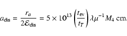 |
(31) |
When
(the cases a1 and a2)
we can obtain an explicit expression for
with the help of (21):
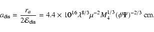 |
(32) |
The condition
 (or
)
can be written as
a condition for the parameter
to be larger than a certain value.
For our discussion below it is more convenient to use the quantity
defined in Eq. (8) instead of .
Depending on which case is considered (i.e. a1, a2 or b2),
the inequality
can be written as a condition that the
quantity
is larger than its values
(or
)
can be written as
a condition for the parameter
to be larger than a certain value.
For our discussion below it is more convenient to use the quantity
defined in Eq. (8) instead of .
Depending on which case is considered (i.e. a1, a2 or b2),
the inequality
can be written as a condition that the
quantity
is larger than its values
 ,
,
 and
and  corresponding to the equality
 for the respective cases. These values are explicitly obtained in the Appendix, see Eq. (A.5) for the case a1, Eq. (A.7) for the case a2 and Eq. (A.10) for the case b2.
6 The rate of tidal capture by the black hole
In order to estimate the rate of tidal capture by the black hole we assume
that the stars in the cusp are slowly rotating. Therefore,
at the beginning of orbital circularisation the effects of rotation
are not important so we neglect it when estimating
the rate of capture into circularising orbits,
setting
in the expression (21) for the time scale of orbital evolution.
Then from the discussion in Sect. 5 and data plotted in Figs. 2 and 3
it follows that during this phase orbital energy loss resulting from tides is more
important than that due to gravitational radiation.
The rate of capture into circularising orbits, as a function of initial
binding energy per unit mass of the star, depends on whether the tidal time scale (21) is larger than the orbital period
 .
Equating (21) to (3) we find the binding energy per unit mass
.
Equating (21) to (3) we find the binding energy per unit mass
 where these two times are equal to be given by
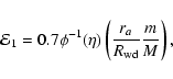 |
(33) |
and we recall the relation between
and the
that applies when
the condition
as given by (11) is fulfilled is
 .
.
At first we assume that
 for a range of angular momenta of interest.
A star gets tidally captured by the black hole
when the characteristic time scale of evolution of its angular
momentum due to distant gravitational encounters with other stars
in the cluster
for a range of angular momenta of interest.
A star gets tidally captured by the black hole
when the characteristic time scale of evolution of its angular
momentum due to distant gravitational encounters with other stars
in the cluster
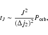 |
(34) |
is larger than the tidal time scale tT (recall that the dispersion of angular momentum j22 is given by Eq. (5)). Equating tJ and tT we find the size of the "tidal
circularisation'' loss cone in angular momentum space as a
function of the dimensionless binding energy ,
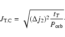 |
(35) |
Note that Eq. (35) defines
 implicitly since this
quantity enters the right hand side through the dependence of tT on
implicitly since this
quantity enters the right hand side through the dependence of tT on  To deal with this we define
 ,
where we recall that
,
where we recall that
 Then we have
 ,
see Eqs. (9) and (10). Using the above,
an equation for
,
see Eqs. (9) and (10). Using the above,
an equation for
 may be obtained from
Eqs. (5), (20) and (35) in the form
may be obtained from
Eqs. (5), (20) and (35) in the form
 |
(36) |
where
 .
It follows from Eq. (20) that in order to find
and hence
the size of the tidal loss cone we need to evaluate
the ratio
.
It follows from Eq. (20) that in order to find
and hence
the size of the tidal loss cone we need to evaluate
the ratio
 when
when
 This quantity grows from small values as the orbital period increases
from small values,
and accordingly the binding energy decreases, until it reaches unity
when
This quantity grows from small values as the orbital period increases
from small values,
and accordingly the binding energy decreases, until it reaches unity
when
 At that point
Eq. (33) applies as well as the condition that
At that point
Eq. (33) applies as well as the condition that
 |
(37) |
These two equations define a critical energy
 .
.
When
 the tidal
evolution time scale is approximately equal to the orbital period
and therefore the size
of the tidal circularisation loss cone is determined by Eq. (33) which is, in this case, considered as an implicit equation
for
the tidal
evolution time scale is approximately equal to the orbital period
and therefore the size
of the tidal circularisation loss cone is determined by Eq. (33) which is, in this case, considered as an implicit equation
for
 for a given value of
 .
Stars with these energies which have
.
Stars with these energies which have
 calculated in this way have relatively large energy changes
induced within a single orbit.
calculated in this way have relatively large energy changes
induced within a single orbit.
When
 the number of stars tidally captured by the
black hole per unit of time, with typical energies of order of
some E,
the number of stars tidally captured by the
black hole per unit of time, with typical energies of order of
some E,
 ,
can be estimated to be
,
can be estimated to be
 |
(38) |
where we assume that the distribution function of the white dwarfs
is given by Eq. (4).
Using Eqs. (2), (5) and (35) we see that, in this case,
 |
(39) |
is mainly determined by stars with small energies. Note that we take into
account the fact that  depends only logarithmically on the binding energy when deriving the relation (39), see Eq. (35).
For the case
it can be easily seen that
 for any value of J.
This situation is analogous to the full loss cone regime
in the theory of tidally disrupted stars (e.g. Frank
Rees
1976; Lightman
Shapiro 1977). In this case the rate of tidally captured stars can be estimated as
for any value of J.
This situation is analogous to the full loss cone regime
in the theory of tidally disrupted stars (e.g. Frank
Rees
1976; Lightman
Shapiro 1977). In this case the rate of tidally captured stars can be estimated as
 |
(40) |
where here we take into account the fact that the size
of loss cone, now implicitly determined by Eq. (33),
depends logarithmically and hence slowly on E.
Thus, the rate of tidal circularisation is mainly determined by
energies
 (Novikov et al. 1992),
and therefore it important to obtain
an explicit expression for the value of
.
As we
discussed above this value is determined by the condition that
the timescale for orbital evolution due to tides be equal to the orbital period
while being on the boundary of the tidal loss cone.
It is determined by Eqs. (33) and (37) which can be rewritten in the form
(Novikov et al. 1992),
and therefore it important to obtain
an explicit expression for the value of
.
As we
discussed above this value is determined by the condition that
the timescale for orbital evolution due to tides be equal to the orbital period
while being on the boundary of the tidal loss cone.
It is determined by Eqs. (33) and (37) which can be rewritten in the form
 |
(41) |
where
 and
and
 is found from Eq. (8) after setting
 ,
together with
,
together with
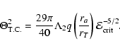 |
(42) |
Substituting
 from (41) to (42) we obtain
a single equation for
and thence
in the form
from (41) to (42) we obtain
a single equation for
and thence
in the form
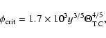 |
(43) |
where
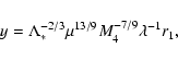 |
(44) |
and
.
Using the explicit expression for
and the relation
 we rewrite (43) in another form
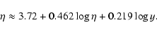 |
(45) |
An approximate solution to Eq. (45) valid for the range
of interest of the parameter
 -10 with accuracy of order of 10 per cent is
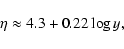 |
(46) |
and
 |
(47) |
As seen from Eq. (47) the size of the tidal
circularisation loss cone given by
corresponding to
the critical energy
is larger than
the size of the tidal disruption loss cone given by  .
.
This is different from the situation where only the effect of emission of gravitational
waves is taken into account as a mechanism for changing the orbital
energy. In that case the energy scale analogous
may also be
obtained from the requirement that the orbital evolution time
 be equal
to the orbital period on the
boundary of the corresponding circularisation loss cone.
Obviously, our estimate of the circularisation rate is valid only when
the size of the circularisation loss cone is larger than the size of "true''
loss cone,
be equal
to the orbital period on the
boundary of the corresponding circularisation loss cone.
Obviously, our estimate of the circularisation rate is valid only when
the size of the circularisation loss cone is larger than the size of "true''
loss cone,
 corresponding to direct capture or disruption of stars by
the black hole.
However, for typical parameters expected for
gravitational waves to be the dominant process of orbital
evolution (
corresponding to direct capture or disruption of stars by
the black hole.
However, for typical parameters expected for
gravitational waves to be the dominant process of orbital
evolution (
 and
and
 )
the energy scale
is smaller than another energy scale
)
the energy scale
is smaller than another energy scale
 defined by the
condition that the sizes of the circularisation and true loss cones coincide
at
defined by the
condition that the sizes of the circularisation and true loss cones coincide
at
 .
When
.
When
 the stars are mainly destroyed by the black hole
and the process of circularisation is strongly suppressed.
In such a situation the capture rate is mainly
determined by energies
the stars are mainly destroyed by the black hole
and the process of circularisation is strongly suppressed.
In such a situation the capture rate is mainly
determined by energies
 (Hopman
Alexander 2005). Because of this difference, the tidal circularisation rate in our case, (see Eq. (51) below) differs
from the estimate of the capture rate due to emission of
gravitational waves provided by Hopman
Alexander (2005), see also Novikov et al. (1992).
(Hopman
Alexander 2005). Because of this difference, the tidal circularisation rate in our case, (see Eq. (51) below) differs
from the estimate of the capture rate due to emission of
gravitational waves provided by Hopman
Alexander (2005), see also Novikov et al. (1992).
Equation (41) gives
 |
(48) |
We have explicitly
 |
(49) |
It is important to note that the critical energy
 for our problem and therefore, the circularisation rate is mainly determined
by scales well within the cusp around the black hole. Also, Eq. (46) tells that
as we have mentioned above.
for our problem and therefore, the circularisation rate is mainly determined
by scales well within the cusp around the black hole. Also, Eq. (46) tells that
as we have mentioned above.
The maximal rate of capture ,
 can be estimated
a little more accurately as
can be estimated
a little more accurately as
 |
(50) |
where
 is given by Eq. (4) with
 and
is defined in Sect. 2.4. Let us recall that
in our problem
and
is defined in Sect. 2.4. Let us recall that
in our problem
 .
Integrating (50) we get
.
Integrating (50) we get
 |
(51) |
where
 |
(52) |
and we assume that
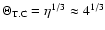 in the last
equality. In astrophysical units the expression (51) has the form
in the last
equality. In astrophysical units the expression (51) has the form
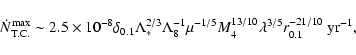 |
(53) |
where
 and
and
 .
Note that we use
.
Note that we use
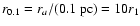 in the last equation
assuming that a typical size of the radius of influence in
globular clusters is of the order of 0.1 pc.
in the last equation
assuming that a typical size of the radius of influence in
globular clusters is of the order of 0.1 pc.
As discussed in Sect. 5,
a white dwarf has a possibility
of surviving the process of circularisation, and accordingly,
settling on a quasi-circular orbit only when a typical value of
the parameter
(or equivalently the pericentre distance)
is sufficiently large.
The tidally captured white dwarfs with formation rate
 have a typical value of
given by Eq. (46) and, accordingly,
have a typical value of
given by Eq. (46) and, accordingly,
 given by Eq. (47).
According to the discussion in Sect. 5 and the Appendix,
such white dwarfs have a considerable survival probability,
for cases a1) and a2) corresponding to large tnl, when
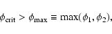 |
(54) |
where
and
are determined by Eqs. (A.5) and (A.7), respectively.
For case b2) corresponding to small
tnl, for survival we require that
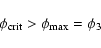 |
(55) |
instead of (54), where
is given by Eq. (A.10).
When the above conditions are not satisfied,
the typical binding energy of white dwarfs having
a considerable probability of survival,  ,
has to be larger than
the critical value obtained from Eq. (49) and so their capture rate
is reduced by a factor
,
has to be larger than
the critical value obtained from Eq. (49) and so their capture rate
is reduced by a factor
 when compared to that given by Eq. (53) (see Eq. (39)). Accordingly their
capture rate is given by
when compared to that given by Eq. (53) (see Eq. (39)). Accordingly their
capture rate is given by
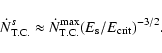 |
(56) |
The binding energy per unit mass, ,
is related to the quantity
 through the "loss cone condition'' (36). Taking
into account the fact that the dependence of
on
and
is logarithmic, we
approximately have
through the "loss cone condition'' (36). Taking
into account the fact that the dependence of
on
and
is logarithmic, we
approximately have
 ,
and therefore
Eq. (56) can be written as
,
and therefore
Eq. (56) can be written as
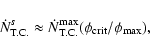 |
(57) |
and accordingly, the rate of formation is suppressed by the factor
 which is less than unity when conditions (54) and (55) are not satisfied. As indicated below that is likely to be the situation for cases of interest.
We go on to obtain explicit expressions for the rate of capture of
white dwarfs that may survive the circularisation process in that case.
This rate will be referred to as "the circularisation rate''.
First let us consider the case a) for which
.
As follows from Eq. (A.8)
 when
when
 .
Since the systems containing sufficiently
massive black holes are likely to provide the bulk of the sources of
gravitational radiation, we assume hereafter that
and set, accordingly,
.
Since the systems containing sufficiently
massive black holes are likely to provide the bulk of the sources of
gravitational radiation, we assume hereafter that
and set, accordingly,
 .
In this case the condition (54) leads to
.
In this case the condition (54) leads to
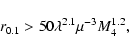 |
(58) |
where we use Eqs. (A.7) and (44). In the
systems of interest this condition is not satisfied, and
indeed the circularisation rate is suppressed.
We use Eqs. (44), (47), (53) and (57) to obtain the
the suppressed capture or circularisation rate in the form
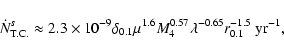 |
(59) |
where hereafter we set the logarithmic factors
 .
Substituting values of
and
appropriate
for a "low density'' white dwarf in (59), we obtain
.
Substituting values of
and
appropriate
for a "low density'' white dwarf in (59), we obtain
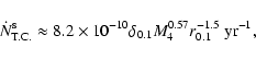 |
(60) |
and in the case of the "high density'' white dwarf with
 and
and  ,
we obtain
,
we obtain
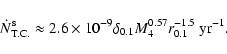 |
(61) |
Now let us consider case b2) for which
 .
In this case the condition (55) can be expressed as
.
In this case the condition (55) can be expressed as
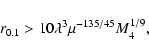 |
(62) |
where we have made use of Eqs. (A.10) and (47).
According to Eq. (62) the circularisation rate
is equal to the rate of tidal capture (53) when the cusp size
is sufficiently large.
For large cusp sizes the circularisation rate becomes
small due to a strong decrease of the capture rate as it increases (see Eq. (53)).
Thus such systems are not likely to contribute significantly
to the total number of gravitational wave sources.
Therefore, we assume hereafter that the inequality (62) does not apply and multiply (53) by the suppression factor
 in
order to obtain the circularisation rate. Thus we have
in
order to obtain the circularisation rate. Thus we have
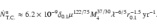 |
(63) |
Substituting values appropriate to the two types of white dwarf in (63), we obtain
for the "low density'' case
 |
(64) |
and
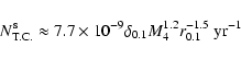 |
(65) |
for the "high density case''.
A comparison of Eq. (53) with Eqs. (59)-(61), (63)-(65) shows that our criterion of survival of the white dwarfs during the process of circularisation typically results
in an order of magnitude decrease of the circularisation rate.
However note that for case b2) when tnl is small, the suppression is not significant for the ``high density'' white dwarfs..
7 Probability of detection of a source of gravitational radiation
The probability of formation of observable sources of gravitational waves
is determined by several important factors such as the rate of formation
of white dwarfs on circularising orbits
calculated above, the subsequent orbital evolution of the white dwarfs,
the abundance
of globular clusters having sufficiently massive black holes
and the properties of a gravitational wave antenna
receiving the signal. In what follows we make
a rough estimate of the probability assuming that the gravitational
wave antenna has characteristics close to what has been indicated for
the future LISA space borne gravitational wave antenna.
LISA has its maximal sensitivity in the frequency range 10-2 Hz for which the dimensionless amplitude of the gravitational
waves, h, can be as small as
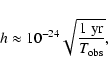 |
(66) |
where
 is the time of observation,
see e.g. Grishchuk et al. (2001, and references therein).
Therefore, for simplicity, we assume that the white dwarf has an
orbital period
is the time of observation,
see e.g. Grishchuk et al. (2001, and references therein).
Therefore, for simplicity, we assume that the white dwarf has an
orbital period
 s
when emitting the gravitational waves to be received by the antenna.
The time
can be smaller than or of the same
order as the orbital evolution
time
s
when emitting the gravitational waves to be received by the antenna.
The time
can be smaller than or of the same
order as the orbital evolution
time
 calculated for an orbital period 100 s,
and we assume hereafter that these are equal to each other,
calculated for an orbital period 100 s,
and we assume hereafter that these are equal to each other,
 .
In order to estimate
we need to specify
a typical value of eccentricity of the orbit, e, which, in turn,
is determined by whether the orbital evolution is governed by tides
or by the emission of the gravitational waves.
For such small orbital periods the evolution is likely to be
determined by the latter effect and we can
use the results obtained by Peters
Mathews (1963) and Peters
(1964) when estimating e. To do that we proceed as follows. First
we estimate the orbital semi-major axis for an orbit with
.
In order to estimate
we need to specify
a typical value of eccentricity of the orbit, e, which, in turn,
is determined by whether the orbital evolution is governed by tides
or by the emission of the gravitational waves.
For such small orbital periods the evolution is likely to be
determined by the latter effect and we can
use the results obtained by Peters
Mathews (1963) and Peters
(1964) when estimating e. To do that we proceed as follows. First
we estimate the orbital semi-major axis for an orbit with
 s from Kepler's law as
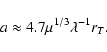 |
(67) |
Next we use the dependence of the orbital angular momentum on e obtained by Peters (1964)
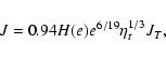 |
(68) |
where
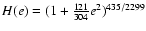 .
Equation (68)
implies that when
.
Equation (68)
implies that when  the orbital angular momentum
is equal to
the orbital angular momentum
is equal to
 .
Since a typical value of
allowing survival
during the process of tidal
circularisation, according to Sect. 5 and Appendix,
is slightly larger than the typical value
.
Since a typical value of
allowing survival
during the process of tidal
circularisation, according to Sect. 5 and Appendix,
is slightly larger than the typical value
 ,
we set
,
we set
 hereafter. Now we can
equate the standard expression
hereafter. Now we can
equate the standard expression
 to
what is given in Eq. (68), and using Eq. (67) with
obtain an implicit equation for the eccentricity e
to
what is given in Eq. (68), and using Eq. (67) with
obtain an implicit equation for the eccentricity e
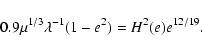 |
(69) |
From this equation we obtain
 and
and
 for the high/low density white dwarfs, respectively.
The evolution time can be expressed
in the form
for the high/low density white dwarfs, respectively.
The evolution time can be expressed
in the form
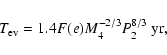 |
(70) |
where
 s and the function F(e) specifies
the dependence of
on e, see Peters (1964).
We have
F(e=0)=1,
s and the function F(e) specifies
the dependence of
on e, see Peters (1964).
We have
F(e=0)=1,
 and
and
 .
Note, that an analogous expression for
given in Ivanov (2002) in his
Eq. (79) contains an error in last expression on the right
hand side and must be multiplied on
additional factor
.
Note, that an analogous expression for
given in Ivanov (2002) in his
Eq. (79) contains an error in last expression on the right
hand side and must be multiplied on
additional factor
 .
As a result, although
his estimate of a probability of finding a source of gravitational
waves in galactic centres containing black holes of masses
.
As a result, although
his estimate of a probability of finding a source of gravitational
waves in galactic centres containing black holes of masses
 (Eq. (80) of his paper)
is numerically correct for the parameters
he uses, it has a different scaling with the black hole mass.
It must be multiplied by an additional factor
which results in smaller values of the probability for
black hole masses in the range 104-
.
(Eq. (80) of his paper)
is numerically correct for the parameters
he uses, it has a different scaling with the black hole mass.
It must be multiplied by an additional factor
which results in smaller values of the probability for
black hole masses in the range 104-
.
Now, substituting (70) in (66) we obtain
minimal values of the amplitude h,  ,
which can
be detected by LISA
,
which can
be detected by LISA
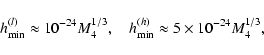 |
(71) |
where
 stands for the minimal amplitudes for the cases of low/high density white dwarfs, respectively, and we set P2=1.
In order to find the total volume of space, available
for detection of the signals by LISA, we should relate the quantities
to the distance from a source,
 .
For that
the amplitude h of radiation emitted by the source should be known
as a function of distance and of parameters of the source.
The appropriate relation has been obtained, e.g., by Nelemans et al. (2001). In our units it has the form
.
For that
the amplitude h of radiation emitted by the source should be known
as a function of distance and of parameters of the source.
The appropriate relation has been obtained, e.g., by Nelemans et al. (2001). In our units it has the form
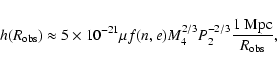 |
(72) |
where the function f(n,e) contains information about the amplitudes
associated with harmonics of different order n. It is related to
the function g(n,e) calculated by Peters
Mathews (1963)
through
 . We have
 for
several harmonics with n=1,2,3 and
for
several harmonics with n=1,2,3 and
 .
Now we can equate
.
Now we can equate
 to
to
 and find the maximal distance to a source which can be, in principal, detected by LISA
 |
(73) |
where the upper indices (l,h) stand for the cases of low/high
density white dwarfs hereafter.
In order to find the total number of potential sources,
 ,
we use an estimate obtained by Portegies Zwart
McMillan (2000) for
the average number of globular clusters in the Universe,
,
we use an estimate obtained by Portegies Zwart
McMillan (2000) for
the average number of globular clusters in the Universe,
 for the value of the Hubble constant
H=70 km s-1 Mpc-1. We obtain from Eq. (73)
for the value of the Hubble constant
H=70 km s-1 Mpc-1. We obtain from Eq. (73)
 |
(74) |
where  is the fraction of globular clusters having black
holes with masses M4. The total probabilities of finding of
a source,
Pr(1,2), can be estimated as products of the circularisation rates
given by Eqs. (60) and (61) for case a) and Eqs. (64) and (65) for case b), the total numbers of the sources available and the operational time of the LISA mission taken to be equal to 2 yr.
is the fraction of globular clusters having black
holes with masses M4. The total probabilities of finding of
a source,
Pr(1,2), can be estimated as products of the circularisation rates
given by Eqs. (60) and (61) for case a) and Eqs. (64) and (65) for case b), the total numbers of the sources available and the operational time of the LISA mission taken to be equal to 2 yr.
For case a) with
,
using Eqs. (60), (61) and (74) we have
 |
(75) |
where
 |
(76) |
It is seen from Eq. (75) that the high density white dwarfs of
Sirius B type give rather small probability of detection. On the other
hand, the "ordinary'' white dwarfs could provide, in principal,
a source of gravitational waves provided that our criterion of white
dwarfs survival is valid and that
 |
(77) |
It is interesting reformulate the criterion (77)
in term of a typical velocity of stars near the radius of influence
of the black hole,
 .
We have from Eqs. (76) and (77)
.
We have from Eqs. (76) and (77)
 |
(78) |
where we neglect a very slow dependence on the black hole mass,
 .
Of course, the black hole mass
must be sufficiently large for the validity of the assumptions
leading to Eq. (77).
.
Of course, the black hole mass
must be sufficiently large for the validity of the assumptions
leading to Eq. (77).
For case b) with
we proceed in a similar manner
but use Eqs. (64) and (65) instead of Eqs. (60) and (61), respectively. We find
 |
(79) |
where
 |
(80) |
and
 |
(81) |
instead of Eq. (78) for a "typical low density'' white dwarf.
As for case a) "typical'' white dwarfs have a much larger probability of detection.
However, for case b) this probability depends explicitly on the black hole mass
when the cusp size is expresses in terms of the typical stellar velocity dispersion  .
As follows from Eqs. (79)-(81) when
.
As follows from Eqs. (79)-(81) when
 and
and
 km s-1 this probability is about
two times larger than that corresponding to case a). But the probability ratio decreases
with the black hole mass if
is kept fixed.
km s-1 this probability is about
two times larger than that corresponding to case a). But the probability ratio decreases
with the black hole mass if
is kept fixed.
8 Discussion
In this paper we have given a qualitative analysis of the problem of tidal
circularisation of white dwarfs in globular clusters containing black
holes with masses in the range 103-
and estimated
the rate of production of
white dwarfs that begin to circularise their orbits
for specified parameters for the cluster, white dwarf and black hole, see Eq. (53). We also
proposed a simple criterion for "survival'' of a white dwarf during
the stage of orbital circularisation, and found production rates for
white dwarfs, which can, in principal, settle down in a
quasi-circular orbit thus forming sources of gravitational radiation,
see Eqs. (59-61) and (63-65).
These rates are order of magnitude
smaller than that given by Eq. (53). We made a simple
estimate of the probability of detection of systems containing
white dwarfs on quasi-circular orbits and found that these systems can,
in principle, be detected by LISA provided that the globular clusters
containing black holes are sufficiently abundant and their stellar velocity
dispersion near the radius of influence of the black hole is
sufficiently large, see Eqs. (78) and (81).
Our results should be treated with caution.
Many processes occurring during the formation of circularising stars
and during ongoing tidal circularisation depend strongly on the parameters
of the problem and this leads to uncertainties in the results.
Let us consider some of them.
- 1)
- In a quantitative approach a realistic model of a white dwarf
with non-zero temperature should be used. The eigen spectrum of
perturbations should include the gravity/inertial modes. The
realistic model should also take into account different channels
of mode decay and a self-consistent change of
structure of the white dwarf
as a result of radiative cooling/heating due to dissipation of the mode
energy.
- 2)
- Our results indicate that the stars can achieve very high rotation
rates during the process of ongoing tidal circularisation. The
possibility of survival of white dwarfs during this stage critically
depends on tidal exchange of energy between the orbit and
the modes of a fast rotating star. It will be very important
to generalise well known results of the theory of dynamic
tides in non-rotating/slowly rotating stars to the
case of fast rotators.
- 3)
- As follows from this discussion, our results depend
on the rate of mode energy and angular momentum transfer to the star.
Possible channels for this transfer, especially
through dissipation resulting from non linear effects should be
further investigated.
- 4)
- The dependence of the circularisation rate on the cusp size
and black hole mass should be checked with
numerical N-body simulations. Also, a more realistic distribution
of the white dwarfs over the cluster as well as a change of
their relative fraction due to stellar evolution should be
accounted for in a numerical study.
- 5)
- We have adopted a rather simplistic criterion for detection
of the gravitational waves produced by the white dwarf orbiting
close to a black hole, assuming that the amplitude of the
signal is equal to the noise amplitude of the detector. Higher
S/N detection threshold would result in a much smaller probability of detection.
On the other hand, a more sophisticated strategy of signal
processing could improve our estimates.
We have shown that during the first stage of orbital circularisation
the orbital energy transferred to the fundamental mode of
stellar pulsations may be radiated away by gravitational waves. That means
that the globular clusters may contain sources of gravitational
radiation with a typical frequency of the order of the eigen frequency
of the fundamental quadrupole mode, of the order of a few Hz.
The possibility of detection of such sources needs further
investigation.
Finally we comment that in a recent paper
Baumgardt et al. (2006) have calculated the tidal capture rates for stars of
different types with help of N-body simulations, during
first 12Myrs of evolution of the system. They have considered
black holes with masses in the range
103-
 .
Giant stars and low mass
main sequence stars with mass <0.4
have been modelled
as n=1.5 polytropes. The low mass stars seem to be absent in the
cusp due to the effect of mass segregation operating
during formation of the cusp.
However, their capture rate of red giants can be compared
with what is given by Eq. (53). They have obtained a capture
rate for red giants of the order of a few events per run.
Assuming that a typical red giant has a radius 10
.
Giant stars and low mass
main sequence stars with mass <0.4
have been modelled
as n=1.5 polytropes. The low mass stars seem to be absent in the
cusp due to the effect of mass segregation operating
during formation of the cusp.
However, their capture rate of red giants can be compared
with what is given by Eq. (53). They have obtained a capture
rate for red giants of the order of a few events per run.
Assuming that a typical red giant has a radius 10
 ,
mass
,
mass
 ,
taking the black hole
mass and the cusp size to be equal to
,
taking the black hole
mass and the cusp size to be equal to
 and to
0.1 pc, respectively, and substituting these values into
Eq. (53), we obtain
and to
0.1 pc, respectively, and substituting these values into
Eq. (53), we obtain
 yr-1, where
 is the number fraction of the red giants in the
cusp. Our results appears to be
in full agreement with the results of N-body simulations provided
that
is the number fraction of the red giants in the
cusp. Our results appears to be
in full agreement with the results of N-body simulations provided
that
 .
.
Acknowledgements
We are grateful to A. G. Polnarev for fruitful discussions to A. G. Doroshkevich for useful remarks and to the referee for valuable comments. P.B.I. has been supported in part by RFBR grants 04-02-17444 and 07-02-00886.
Appendix A: Conditions for the transition from stochastic instability
As indicated in Sect. 3.7, there is a phase of evolution
at large semi-major axis subsequent to tidal capture
where the internal pulsation mode energy may increase in a stochastic manner.
This requires the semi-major axis to exceed
 above which
the pulsation mode does not maintain phase coherence
between successive pericentre passages.
above which
the pulsation mode does not maintain phase coherence
between successive pericentre passages.
Here we obtain an explicit expression for the semi-major axis
defined through Eq. (13). At first let us assume that
 during the orbital
evolution. This situation is illustrated in Figure 2. In this case we substitute Eq. (7) in
Eq. (13) and obtain
during the orbital
evolution. This situation is illustrated in Figure 2. In this case we substitute Eq. (7) in
Eq. (13) and obtain
 |
(A.1) |
Now let us consider the orbital evolution when
 .
This situation is illustrated in Figure 1.
In this case the semi-major corresponding to the onset
of the stochastic instability,
.
This situation is illustrated in Figure 1.
In this case the semi-major corresponding to the onset
of the stochastic instability,
 can be obtained by substitution of Eq. (28)
in Eq. (13) with the result
can be obtained by substitution of Eq. (28)
in Eq. (13) with the result
 |
(A.2) |
Just after tidal capture occurs the orbital evolution is primarily due to
tides. The orbit decays until
is reached but at this point
it is possible that the orbital evolution is governed by gravitational
radiation. As indicated in Sect. 5, when the orbital
semi-major axis is of the order of
there are three non trivial
possibilities:
case a1) where
and tides determine the orbital
evolution; case a2) where
and gravitational radiation determines the orbital
evolution; and case b2) where
and gravitational radiation controls the orbital
evolution. Each of these is considered in more detail below.
A.1 The case a1: tides dominate and t
 is large
As indicated in Sects. 4 and 5, when
a white dwarf has a possibility of surviving
the process of tidal circularisation only if it is cooled
efficiently by emission of gravitational waves for
values of its semi-major axes >
 .
Therefore, in order
to reach a quasi-circular orbit, the white dwarf must have orbital parameters
such that
.
Therefore, in order
to reach a quasi-circular orbit, the white dwarf must have orbital parameters
such that
 where
is given by
Eq. (32). This inequality leads to an inequality of the form
where
is given by
Eq. (32). This inequality leads to an inequality of the form
 (or equivalently the fixed pericentre distance must exceed a certain value),
where
(or equivalently the fixed pericentre distance must exceed a certain value),
where  is defined by the condition
 .
In general, is a monotonic function of the stellar rotation rate with smaller values of corresponding to larger values of
.
This is because tides
weaken with increasing
enabling safe circularisation
starting with smaller pericentre distances.
.
In general, is a monotonic function of the stellar rotation rate with smaller values of corresponding to larger values of
.
This is because tides
weaken with increasing
enabling safe circularisation
starting with smaller pericentre distances.
Thus in order to take into account all possible evolutionary
tracks leading to formation of circular orbits, we calculate the lower
boundary of
assuming that
 .
In this case the
factor
.
In this case the
factor
 entering (A.1) takes the form
 |
(A.3) |
Substituting Eq. (A.3) in Eq. (A.1) and Eqs. (32) and (A.1), we obtain
 |
(A.4) |
where
 .
.
In the subsequent discussion we
use the quantity
 defined in Eq. (8)
rather than .
This quantity can be approximately represented
in the form
defined in Eq. (8)
rather than .
This quantity can be approximately represented
in the form
 |
(A.5) |
with the difference between this power-law fit and the solution of
Eq. (A.4) being less than or of the order of 5 per cent
for all interesting values of Z1.
A.2 The case a2: gravitational waves dominate
and
 is large
Now let us assume that gravitational waves determine the orbital evolution
when a rapidly rotating white dwarf has its semi-major axis near to
and
 ,
see Fig. 1. Proceeding as in the preceding section, we
obtain an equation for the critical value of
,
see Fig. 1. Proceeding as in the preceding section, we
obtain an equation for the critical value of  that is analogous to Eq. (A.4) in the form
 |
(A.6) |
where
 .
The corresponding value of
.
The corresponding value of
 can also be, with a high accuracy, represented in the power-law form
 |
(A.7) |
The value of the parameter
and thus
which divides, according to our criterion,
orbits leading to a safe circularisation
from orbits leading to a possible disruption of the white dwarf,
is obtained from the condition
 .
We note that the condition for gravitational
radiation to dominate,
,
leads to the approximate condition on the black hole mass that
.
We note that the condition for gravitational
radiation to dominate,
,
leads to the approximate condition on the black hole mass that
 |
(A.8) |
where we have neglected a very weak dependence of M* on
of the form
 the latter quantity being replaced by unity.
The inequality (A.8) implies that for a sufficiently large
values of the black hole mass and the rotation of the white
dwarf the orbital evolution is mainly determined by emission
of gravitational waves when the semi-major of the orbit
is close to the characteristic semi-major axis corresponding to the onset
of stochastic instability. For the parameters corresponding
to a "typical'' white dwarf with
and
,
we have
 ,
and for a dense white dwarf of Sirius B type with and
,
we have
M*=0.13. Both characteristic values
of M* are smaller than the black hole masses of
systems expected to produce a large amount of gravitational
radiation during the last stages of orbital evolution of the star.
Therefore, the condition
,
and for a dense white dwarf of Sirius B type with and
,
we have
M*=0.13. Both characteristic values
of M* are smaller than the black hole masses of
systems expected to produce a large amount of gravitational
radiation during the last stages of orbital evolution of the star.
Therefore, the condition
 is more important for
our purposes.
is more important for
our purposes.
A.3 The case b2: gravitational waves dominate and t is small
Now let us consider the case when
.
The discussion
proceeds in a similar way to the previous case but now
is given by Eq. (31). As we have mentioned above
it can then be shown that gravitational waves dominate the orbital evolution
when the semi-major axis is
provided that the black hole mass exceeds
 ,
and accordingly,
.
,
and accordingly,
.
Therefore in order to obtain an equation for the parameter
 separating orbits leading to safe circularisation from those
leading to disruption of the star, we equate expressions (31) and (A.2),
and use Eqs. (7), (28), (29) and (A.3),
to obtain
separating orbits leading to safe circularisation from those
leading to disruption of the star, we equate expressions (31) and (A.2),
and use Eqs. (7), (28), (29) and (A.3),
to obtain
 |
(A.9) |
where
 .
An approximate solution to this equation can be found from
.
An approximate solution to this equation can be found from
 |
(A.10) |
- Bahcall, J.
N., & Wolf, R. A. 1976, ApJ, 209, 214 [NASA ADS] [CrossRef]
(In the text)
-
Baumgardt, H., Makino, J., & Ebisuzaki, T. 2004a, ApJ, 613,
1133 [NASA ADS] [CrossRef]
-
Baumgardt, H., Makino, J., & Ebisuzaki, T. 2004b, ApJ, 613,
1144 [NASA ADS]
-
Baumgardt, H., Hopman, C., Portegies Zwart, S. F., & Makino, J.
2006, MNRAS, 372, 467 [NASA ADS]
(In the text)
- Chugunov,
A. I., & Yakovlev, D. G. 2005, Astron. Rep., 49, 724 [NASA ADS] [CrossRef]
(In the text)
- Clement, M.
J. 1989, ApJ, 339, 1022 [NASA ADS] [CrossRef]
(In the text)
- Fabbiano,
G. 1989, A&ARv, 27, 87
(In the text)
- Frank, J., &
Rees, M. J. 1976 MNRAS, 176, 633
(In the text)
- Freitag, M.
2000, ApJ, L21
- Frolov, V. P.,
Khokhlov, A. M., Novikov, I. D., & Pethick, C. J. 1994, ApJ,
432, 680 [NASA ADS] [CrossRef]
(In the text)
- Gebhardt,
K., Pryor, C., O'Connel, R. D., Williams, T. B., & Hesser, J.
E. 2000, AJ, 119, 1268 [NASA ADS] [CrossRef]
(In the text)
- Gebhardt,
K., Rich, R. M., & Ho, L. C. 2002, ApJ, 578, L41 [NASA ADS] [CrossRef]
(In the text)
- Ghosh, K. K.,
Suleymanov, V., Bikmaev, I., Shimansky, S., & Sakhibullin, N.
2006, MNRAS, 371, 1587 [NASA ADS]
(In the text)
-
Goldreich, P., & Nicholson, P. D. 1989, ApJ, 342, 1075 [NASA ADS] [CrossRef]
(In the text)
-
Grishchuck, L. P., Lipunov, V. M., Postnov, K. A., Prokhorov, M.
E., & Sathyaprakash, B. S. 2001, Physics-Uspekhi, 44, 1
- Gurevich, A.
V. 1964, Geomagnetism and Aeronomy, 4, 192
(In the text)
- Hopman, C.,
& Alexander, T. 2005, ApJ, 629, 362 [NASA ADS] [CrossRef]
(In the text)
- Ivanov, P. B.
2002, MNRAS, 336, 373 [NASA ADS]
(In the text)
- Ivanov, P. B.,
& Novikov, I. D. 2001, ApJ, 549, 467 [NASA ADS] [CrossRef]
(In the text)
- Ivanov, P. B.,
& Papaloizou, J. C. B. 2004, MNRAS, 347, 437 [NASA ADS]
(In the text)
- Kochanek,
C. S. 1992, ApJ, 385, 604 [NASA ADS] [CrossRef]
(In the text)
-
Kosovichev, A. G., & Novikov, I. D. 1992, MNRAS, 258, 715 [NASA ADS]
- Lai, D. 1997, ApJ,
490, 847 [NASA ADS] [CrossRef]
(In the text)
- Lightman,
A. P., & Shapiro, S. L. 1977, ApJ, 211, 244 [NASA ADS] [CrossRef]
(In the text)
- Lee, H. M., &
Ostriker, J. B. 1966, ApJ, 310, 176 [NASA ADS] [CrossRef]
- Managan, R.
A. 1986, ApJ, 309, 598 [NASA ADS] [CrossRef]
- Mardling,
R. A. 1995, ApJ, 450, 722 [NASA ADS] [CrossRef]
(In the text)
-
Matsumoto, H., Tsuru, T. G., & Koyama, K. 2001, ApJ, 547,
L25 [NASA ADS] [CrossRef]
(In the text)
- Miller, C. M.,
& Hamilton, D. P. 2002, MNRAS, 330, 232 [NASA ADS]
(In the text)
- Nelemans,
G., Yungelson, L. R., & Portegies Zwart, S. F. 2001, A&A,
375, 890 [NASA ADS] [CrossRef] [EDP Sciences]
(In the text)
- Novikov, I.
D., Pethick, C. J., & Polnarev, A. G. 1992, MNRAS, 225,
276 [NASA ADS]
(In the text)
- Osaki, Y., &
Hansen, C. J. 1973, ApJ, 277
(In the text)
-
Papaloizou, J. C. B., & Ivanov, P. B. 2005, MNRAS, 364,
L66 [NASA ADS]
(In the text)
- Peters, P. C.
1964, Phys. Rev., 136, 1224 [NASA ADS] [CrossRef]
(In the text)
- Peters, P. C.,
& Mathews, J. 1963, Phys. Rev., 131, 435 [NASA ADS] [CrossRef]
(In the text)
- Portegies
Zwart, S. F., & Mc Milllan, S. L. W. 2000, ApJ, 528, L17 [NASA ADS] [CrossRef]
- Press, W. H.,
& Teukolsky, S. A. 1977, ApJ, 213, 183 [NASA ADS] [CrossRef]
(In the text)
- van
der Marel, R. P. 2004, in Coevolution of Black Holes and Galaxies,
from Carnegie Observatories Centennial Symposia (Cambridge
University Press as Part of the Carnegie Observatories Astrophysics
Series), ed. L. C. Ho, 37
(In the text)
- Young, P. 1980,
ApJ, 242, 1232 [NASA ADS] [CrossRef]
(In the text)
Copyright ESO 2007
![\begin{figure}
\par\includegraphics[width=8cm,clip]{7105fig1.eps}\end{figure}](/articles/aa/full/2007/46/aa7105-07/img26.gif)
![\begin{figure}
\par\includegraphics[width=8cm,clip]{7105fig2.eps}\end{figure}](/articles/aa/full/2007/46/aa7105-07/img153.gif)
![\begin{figure}
\par\includegraphics[width=8cm,clip]{7105fig3.eps}\end{figure}](/articles/aa/full/2007/46/aa7105-07/img157.gif)