| (1) |
A&A 474, 145-154 (2007)
DOI: 10.1051/0004-6361:20077653
J.-P. Zahn1 - A. S. Brun2,1 - S. Mathis3,2,1
1 - LUTH, Observatoire de Paris, CNRS, Université Paris-Diderot; Place Jules Janssen, 92195 Meudon, France
2 -
DSM/DAPNIA/Service d'Astrophysique, CEA Saclay, 91191 Gif-sur-Yvette, France; AIM, UMR 7158, CEA - CNRS - Université Paris 7, France
3 -
Observatoire de Genève, 51 chemin des maillettes, 1290 Sauverny, Switzerland
Received 16 April 2007 / Accepted 18 July 2007
Abstract
Context. We examine the MHD instabilities arising in the radiation zone of a differentially rotating star, in which a poloidal field of fossil origin is sheared into a toroidal field.
Aims. We focus on the non-axisymmetric instability that affects the toroidal magnetic field in a rotating star, which was first studied by Pitts and Tayler in the non-dissipative limit. If such an instability were able to mix the stellar material, it could have an impact on the evolution of the star. According to Spruit, it could also drive a dynamo.
Methods. We compare the numerical solutions built with the 3-dimensional ASH code with the predictions drawn from an analytical study of the Pitts & Tayler instability.
Results. The Pitts & Tayler instability is manifestly present in our simulations, with its conspicuous m=1 dependence in azimuth. But its analytic treatment used so far is too simplified to be applied to the real stellar situation. Although the instability generated field reaches an energy comparable to that of the mean poloidal field, that field seems unaffected by the instability: it undergoes Ohmic decline, and is neither eroded nor regenerated by the instability. The toroidal field is produced by shearing the poloidal field and it draws its energy from the differential rotation. The small scale motions behave as Alfvén waves; they cause negligible eddy-diffusivity and contribute little to the net transport of angular momentum.
Conclusions. In our simulations we observe no sign of dynamo action, of either mean field or fluctuation type, up to a magnetic Reynolds number of 105. However the Pitts & Tayler instability is sustained as long as the differential rotation acting on the poloidal field is able to generate a toroidal field of sufficient strength. But in the Sun such a poloidal field of fossil origin is ruled out by the nearly uniform rotation of the deep interior.
Key words: instabilities - stars: magnetic fields - stars: rotation - magnetohydrodynamics (MHD)
Spruit (1999, 2002) analyzed the latter instability in more detail, including Ohmic dissipation and radiative damping, and starting from the dispersion relation established by Acheson (1978); he suggested that it could regenerate the toroidal field, and thus drive a genuine dynamo. Applying essentially Spruit's prescriptions, Maeder & Meynet (2003, 2004, 2005), Eggenberger et al. (2005) and Heger et al. (2005) introduced this dynamo, and the turbulent transport believed to be associated with it, in their stellar evolution calculations. It proved extremely efficient in establishing quasi uniform rotation. In the case of massive stars, it would increase the loss of angular momentum through the stellar wind, and lead to slower rotating stellar cores; this would yield pulsar rotation rates that are in better agreement with the observations.
However, guided by other observational evidence, Denissenkov & Pinsonneault (2006) questioned the existence of such a powerful process of angular momentum transport; they noticed some inconsistencies in Spruit's heuristic argumentation, which they tried to correct. Unfortunately the choice they made was in conflict with the rigorous analytical treatment of the instability; this was pointed out by Spruit (2006), and that part of their discussion was deleted in the final version (Denissenkov & Pinsonneault 2007). In the meanwhile, Braithwaite (2006) conducted a numerical experiment which he claimed to validate Spruit's dynamo scenario.
Our interest in those instabilities was aroused when we observed them while verifying if a fossil field was able to prevent the spread of the solar tachocline, as had been proposed by Gough & McIntyre (1998): the results of these three-dimensional simulations are reported in Brun & Zahn (2006). We then wanted to check whether these calculations agreed with Spruit's analytical predictions, and this incited us to re-examine his original derivation.
We begin by extending Acheson's dispersion relation to the case where both an entropy gradient and a composition gradient are present, and derive the actual solutions of that equation (rather than upper or lower bounds). We then discuss the heuristic arguments that were first used by Spruit, and show how they can be misleading. Next we compare the analytical solutions with the numerical results obtained in Brun & Zahn (2006, hereafter referred to as BZ06), and finally we examine whether the dynamo that was suggested by Spruit does actually operate.
As was done in previous works, we perform a local analysis and examine the stability of an imposed axisymmetric toroidal field. We submit it to wave-like perturbations of the form
| (1) |
 |
(3) |
 |
(4) |
![\begin{displaymath}\zeta^2+4\zeta-[m^2 (1+A)-2(p+1)]=0 .
\end{displaymath}](/articles/aa/full/2007/40/aa7653-07/img42.gif) |
(5) |
 |
(6) |
We consider here only the case where the Roberts number
![]() may be treated as a small quantity, which is the case in stellar interiors (
may be treated as a small quantity, which is the case in stellar interiors (
![]() below the solar convection zone). In Appendix, we derive Acheson's dispersion relation in the more general case where both a gradient of entropy and of chemical composition are present. Then the stratification is characterized by two buoyancy frequencies:
below the solar convection zone). In Appendix, we derive Acheson's dispersion relation in the more general case where both a gradient of entropy and of chemical composition are present. Then the stratification is characterized by two buoyancy frequencies:
 |
(9) |
In Appendix (Eq. (A.15))
we show that the scaled complex frequency
![]() obeys the following third-order equation:
obeys the following third-order equation:
Table 1:
Maximum scaled growth-rate
![]() and corresponding frequency
and corresponding frequency
![]() ,
A* and S, at given
,
A* and S, at given
![]() and for |m|=1.
and for |m|=1.
We observe that if S,
![]() and/or
and/or ![]() ,
are of order unity, this will also be the case for
,
are of order unity, this will also be the case for ![]() ,
which implies that both the frequency
,
which implies that both the frequency
![]() and the growth-rate
and the growth-rate
![]() scale as
scale as
![]() ,
like in the non-dissipative case. The maximum growth-rate and the corresponding frequency are given in Table 1 for a sample of values of
,
like in the non-dissipative case. The maximum growth-rate and the corresponding frequency are given in Table 1 for a sample of values of
![]() ;
we see that it is the prograde mode that is unstable (or rather overstable), except for
;
we see that it is the prograde mode that is unstable (or rather overstable), except for ![]() .
.
For given ratio ![]() ,
the instability domain can be delineated in the [A*, S] plane by locating the points where the growth-rate vanishes and thus where the oscillation frequency is purely real:
,
the instability domain can be delineated in the [A*, S] plane by locating the points where the growth-rate vanishes and thus where the oscillation frequency is purely real:
![]() .
Referring back to (10), this occurs when the following equations are both satisfied:
.
Referring back to (10), this occurs when the following equations are both satisfied:
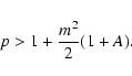
Let us first examine the two limit cases (At=0 and ![]() )
that were considered by Spruit.
)
that were considered by Spruit.
| (13) |
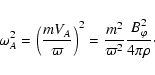
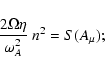
We now use this result to determine the instability threshold. Like Spruit (1999), we eliminate n2 by combining the definition of ![]() :
:
 |
(15) |
![\begin{figure}
\par\includegraphics[width=7.8cm,clip]{7653fig1.eps}
\end{figure}](/articles/aa/full/2007/40/aa7653-07/img87.gif) |
Figure 1:
Limits of the instability domain in the (A*, S) plane, for various values of |
| Open with DEXTER | |
Proceeding as before, we find that the instability threshold is given by
![\begin{displaymath}[\varepsilon A_t~ S(\varepsilon A_t)]~ \omega_A^4 = 2 \Omega \varepsilon \eta l^2 N_t^2 ;
\end{displaymath}](/articles/aa/full/2007/40/aa7653-07/img90.gif) |
(17) |
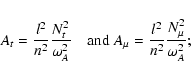
Table 2:
Stratification parameters and optimal conditions for the onset of instability.
![]() is the highest value of
is the highest value of
![]() that allows for instability;
that allows for instability;
![]() the maximum of the product A*S(A*) for fixed
the maximum of the product A*S(A*) for fixed
![]() ,
obtained at
,
obtained at
![]() ,
from which one derives the instability threshold for the magnetic field (see text).
,
from which one derives the instability threshold for the magnetic field (see text).
To determine the instability threshold for the toroidal field, we eliminate as before n2 between
 |
(19) |
For either
![]() or
or ![]() ,
we retrieve the two special cases considered before.
,
we retrieve the two special cases considered before.
In his seminal paper, Spruit (1999) used a few heuristic arguments to describe the Pitts & Tayler instability in a simple, intuitive way. Let us examine their validity in the light of the rigorous treatment given in the preceding section and in Appendix.
With one such arguments, Spruit seeks a lower limit for the vertical wavenumber n. We quote him: "For displacements of amplitude ![]() ,
the work done per unit mass against the stable stratification is
,
the work done per unit mass against the stable stratification is
![]() .
The energy gained from the field configuration is
.
The energy gained from the field configuration is
![]() .
For instability, the field must be strong enough, such that
.
For instability, the field must be strong enough, such that
![]() ''. Furthermore, since
''. Furthermore, since
![]() ,
this provides him a lower limit for n (cf. his Eq. (44)).
,
this provides him a lower limit for n (cf. his Eq. (44)).
In Spruit (2002), the argument is slightly different: ![]() is the unstable displacement, and
is the unstable displacement, and
![]() the kinetic energy that is released in this displacement, "since the growth-rate of the instability in the absence of constraints like rotation is
the kinetic energy that is released in this displacement, "since the growth-rate of the instability in the absence of constraints like rotation is
![]() ''.
''.
Another argument is used to set an upper limit to n: the growth-rate ![]() has to overcome the damping rate of Ohmic diffusion; hence
has to overcome the damping rate of Ohmic diffusion; hence
Denissenkov & Pinsonneault (2006) object quite understandably to this ambivalent choice of ![]() ,
namely
,
namely
![]() for the lower bound and
for the lower bound and
![]() for the upper bound on n. They take the latter definition in both cases, which seems more coherent - but disagrees with the rigorous treatment.
for the upper bound on n. They take the latter definition in both cases, which seems more coherent - but disagrees with the rigorous treatment.
Where is the problem? In fact buoyancy and magnetic field act both as restoring forces, as is illustrated by the energy equation, which we establish in Appendix in the non-dissipative
case (A.22):
These shortcomings of the heuristic approach have been implicitly recognized in Spruit (2006), where he writes that "all physical effects contribute if all terms and factors [meaning
![]() and
and ![]() in our notation] are of the same order [i.e. of order unity, as can be seen in (10)]''. To achieve this, the ratio (l/n)2 has thus to satisfy
in our notation] are of the same order [i.e. of order unity, as can be seen in (10)]''. To achieve this, the ratio (l/n)2 has thus to satisfy
![]() ,
a condition that is less stringent than Spruit's original inequality.
,
a condition that is less stringent than Spruit's original inequality.
The other heuristic condition (21) deserves also a couple of remarks. First, as we show in Appendix, in the limit of small n2 the growth-rate is proportional to the damping rate:
![]() (cf. A.16), and it is not clear what information can be extracted then about n2 by equating these two rates. Second, in presence of radiative damping, why should this condition not be replaced by
(cf. A.16), and it is not clear what information can be extracted then about n2 by equating these two rates. Second, in presence of radiative damping, why should this condition not be replaced by
![]() ,
since the thermal
diffusivity
,
since the thermal
diffusivity ![]() largely exceeds the Ohmic diffusivity?
largely exceeds the Ohmic diffusivity?
We conclude that heuristic arguments, though appealing, can be misleading when they are not supported by a rigorous treatment.
We now come to the suggestion made by Spruit (2002), that this instability could sustain a dynamo in stellar radiation zones, as thermal convection does in a convection zone. We find his idea quite interesting, but we argue that this dynamo cannot operate as he describes it.
According to him, the instability-generated small scale field, which has zero average, is wound up by the differential rotation "into a new contribution to the azimuthal field. This again is unstable, thus closing the dynamo loop''. But this shear induced azimuthal field has the same azimuthal wavenumber as the instability-generated field,
i.e. ![]() and predominantly m =1: it has no mean azimuthal component, and thus it cannot regenerate the mean toroidal field that is required to sustain the instability.
For the same reason, the instability-generated field cannot regenerate the mean poloidal field, as was suggested by Braithwaite (2006). Therefore the Pitts & Tayler instability cannot be the cause of a dynamo, as it was described by Spruit and Braithwaite.
and predominantly m =1: it has no mean azimuthal component, and thus it cannot regenerate the mean toroidal field that is required to sustain the instability.
For the same reason, the instability-generated field cannot regenerate the mean poloidal field, as was suggested by Braithwaite (2006). Therefore the Pitts & Tayler instability cannot be the cause of a dynamo, as it was described by Spruit and Braithwaite.
![\begin{figure}
\par\includegraphics[width=8cm,clip]{7653fig2.eps}
\end{figure}](/articles/aa/full/2007/40/aa7653-07/img121.gif) |
Figure 2:
How to close the dynamo loop involving the Pitts &Tayler instability. In dashed lines the loops proposed by Spruit (A) and Braithwaite (B). The only possible way to regenerate the mean toroidal and/or poloidal field is through the mean electromotive force
|
| Open with DEXTER | |
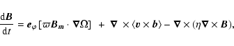
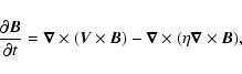
To close the dynamo loop, as is well known in mean-field theory (Parker 1955; Moffatt 1978), one has to invoke the so-called ![]() -effect, which involves the non-zero mean electromotive force
-effect, which involves the non-zero mean electromotive force
![]() that is produced here by the Pitts & Tayler instability. This can be read in the azimuthally averaged induction equation:
that is produced here by the Pitts & Tayler instability. This can be read in the azimuthally averaged induction equation:
 |
(23) |
Another type of dynamo has been observed in numerical simulations, with externally forced turbulence: it is the small-scale or fluctuation dynamo. There the magnetic field has no mean components, neither poloidal nor toroidal, but a quasi-stationary regime may be achieved when the magnetic Reynolds number
![]() exceeds some critical value (V and L are the characteristic velocity and length-scale of the turbulence).
But it remains to be checked whether such a dynamo can be sustained by an imposed shear, such as a differential rotation.
exceeds some critical value (V and L are the characteristic velocity and length-scale of the turbulence).
But it remains to be checked whether such a dynamo can be sustained by an imposed shear, such as a differential rotation.
Table 3: Typical values of the relevant parameters in the upper radiation zone of the Sun, and values adopted for the numerical simulations (in cgs units).
Our simulations, together with the equations of the problem and the resolution methods, are described in full detail in BZ06. We used the global ASH code (Clune et al. 1999;
Brun et al. 2004) to solve the relevant anelastic MHD equations
(Eqs. (1)-(5) in BZ06) in a spherical shell representing the upper part of the solar radiation zone (
![]() ), using a resolution of
), using a resolution of
![]() .
For numerical reasons, we had to increase substantially the diffusivities of heat, magnetic field and momentum, as shown in Table 3, while respecting their hierarchy in the solar conditions. The characteristic evolution times are shortened accordingly, but contrary to BZ06 we made no effort here to rescale them by the Eddington-Sweet time in order to facilitate the comparison with the real Sun. In addition to the case A discussed in BZ06, we performed an additional series of simulations with a lower Ohmic diffusivity (by a factor of 10, case B), in order to reach a higher magnetic Reynolds number.
.
For numerical reasons, we had to increase substantially the diffusivities of heat, magnetic field and momentum, as shown in Table 3, while respecting their hierarchy in the solar conditions. The characteristic evolution times are shortened accordingly, but contrary to BZ06 we made no effort here to rescale them by the Eddington-Sweet time in order to facilitate the comparison with the real Sun. In addition to the case A discussed in BZ06, we performed an additional series of simulations with a lower Ohmic diffusivity (by a factor of 10, case B), in order to reach a higher magnetic Reynolds number.
![\begin{figure}
\par\includegraphics[width=7.4cm,clip]{7653fig3.ps}
\end{figure}](/articles/aa/full/2007/40/aa7653-07/img139.gif) |
Figure 3:
Time evolution of the energies of the mean poloidal (PME), mean toroidal (TME) and non-axisymmetric (FME) components of the magnetic field. Cases A and B refer respectively to higher and lower magnetic diffusivity (cf. Table 3). Note the steady decline of the poloidal field, which is not affected by the irruption of the m=1 Pitts & Tayler instability (at
|
| Open with DEXTER | |
The temporal evolution of the magnetic fields and of the MHD instabilities is best followed in Fig. 3, where we display the energies of the poloidal, toroidal and non-axisymmetric components of the field.
Initially a purely poloidal field of about 1 kG (when measured at the base of the computational domain) is buried in the radiation zone; it is unstable to non-axisymmetric perturbations of high azimuthal wavenumber (
![]() ), as shown in BZ06 (cf. their Fig. 7), which is in agreement with the predictions of Markey & Tayler (1973).
The poloidal field diffuses outward at a rate proportional to the Ohmic diffusivity and at some point (around 8000 days in case A or 20 000 days in case B) it meets the differential rotation that has spread into the radiation zone, due to thermal diffusion. Their interaction induces there a toroidal field, whose strength is comparable to that of the poloidal field in case A; it becomes even larger in case B, where it keeps growing when we stop the simulation, at 60 000 days (corresponding to 1.3 Gyr when rescaled to the Ohmic diffusivity of the Sun).
This toroidal field produces a strong non-axisymmetric MHD instability, with a dominant azimuthal wavenumber m=1, which is clearly the signature of the Pitts & Tayler instability: it is illustrated in Fig. 4. In case A, this instability-generated field saturates at an energy comparable to that of the mean poloidal field, whereas in case B it is still increasing when we stop the simulation, much like the toroidal field.
), as shown in BZ06 (cf. their Fig. 7), which is in agreement with the predictions of Markey & Tayler (1973).
The poloidal field diffuses outward at a rate proportional to the Ohmic diffusivity and at some point (around 8000 days in case A or 20 000 days in case B) it meets the differential rotation that has spread into the radiation zone, due to thermal diffusion. Their interaction induces there a toroidal field, whose strength is comparable to that of the poloidal field in case A; it becomes even larger in case B, where it keeps growing when we stop the simulation, at 60 000 days (corresponding to 1.3 Gyr when rescaled to the Ohmic diffusivity of the Sun).
This toroidal field produces a strong non-axisymmetric MHD instability, with a dominant azimuthal wavenumber m=1, which is clearly the signature of the Pitts & Tayler instability: it is illustrated in Fig. 4. In case A, this instability-generated field saturates at an energy comparable to that of the mean poloidal field, whereas in case B it is still increasing when we stop the simulation, much like the toroidal field.
![\begin{figure}
\par\includegraphics[width=8cm,clip]{7653fig4.eps}
\end{figure}](/articles/aa/full/2007/40/aa7653-07/img142.gif) |
Figure 4:
Azimuthal component of the instability-generated magnetic field, at the peak of the instability ( |
| Open with DEXTER | |
![\begin{figure}
\par\includegraphics[width=7.4cm,clip]{7653fig5CMJN.eps}
\end{figure}](/articles/aa/full/2007/40/aa7653-07/img143.gif) |
Figure 5:
Mean toroidal field
|
| Open with DEXTER | |
Another property of the analytical model is that the vertical wavenumber largely exceeds the horizontal wavenumber, particularly when the stratification is dominated by the ![]() -gradient, since
-gradient, since
![]() (Eq. (14)). In our model, the contrast n/l is less severe, because there is no composition gradient: the instability threshold is then given by (18), which we rewrite here as
(Eq. (14)). In our model, the contrast n/l is less severe, because there is no composition gradient: the instability threshold is then given by (18), which we rewrite here as
 |
(24) |
Therefore we must conclude that the analytical model considered by Spruit is not applicable to the more realistic problem treated in BZ06, and to the situation arising in stars. There may be several reasons for this. The first is that this simplified model ignores the presence of the poloidal field. However its inclusion would probably tend to stabilize the configuration, and that would worsen the discrepancy.
Second, the rotation is taken as uniform, whereas the shear of the differential rotation certainly plays a destabilizing role. Moreover, it is that neglected differential rotation which is the very cause of the instability by generating the toroidal field, a point that has been stressed by Maeder & Meynet (2003).
The third reason is that the ![]() dependence of the instability is poorly described by a trigonometric function, unless the wavelength is small compared to the distance to the axis:
dependence of the instability is poorly described by a trigonometric function, unless the wavelength is small compared to the distance to the axis:
![]() .
Bessel functions would probably be better suited (cf. Tayler 1957).
.
Bessel functions would probably be better suited (cf. Tayler 1957).
Finally the simplified model ignores the curvature effects, as was emphasized by Denissenkov & Pinsonneault (2006). The neglect of the ![]() -component of the buoyancy force, compared to that of the Lorentz force, is allowed only as long as
-component of the buoyancy force, compared to that of the Lorentz force, is allowed only as long as
![]() ,
hence in close vicinity of the rotation axis, for
,
hence in close vicinity of the rotation axis, for
![]() .
This is a very severe restriction, since
.
This is a very severe restriction, since
![]() in our numerical solution (case A).
in our numerical solution (case A).
An important property of our numerical solutions is that the decline of the poloidal field is not affected by the instability-generated field.
As can be seen in Fig. 3, this is true even once the (Pitts & Tayler) instability has reached its saturation level, where its energy is comparable with that of the mean poloidal field. This has two consequences. First it proves that the smallest resolved scales do not act on the mean poloidal field as a turbulent diffusivity: they seem to behave rather as gravito-Alfvén waves, with their kinetic energy balancing their potential energy (magnetic + buoyancy), as in the linear regime described by Eq. (22). Hence the saturation of the instability is not due to the mechanism suggested by Spruit (2002), which was inspired by thermal convection, namely that the magnetic eddy-diffusivity ![]() adjusts such as to neutralize the Pitts & Tayler instability, i.e. that it satisfies Eq. (20). In our model - and presumably also in stellar radiation zones - the regulation is apparently achieved through the action of the Lorentz torque on the differential rotation, which produces just the right amount of toroidal field that is required to sustain the instability, through small departures from Ferraro's law.
adjusts such as to neutralize the Pitts & Tayler instability, i.e. that it satisfies Eq. (20). In our model - and presumably also in stellar radiation zones - the regulation is apparently achieved through the action of the Lorentz torque on the differential rotation, which produces just the right amount of toroidal field that is required to sustain the instability, through small departures from Ferraro's law.
At saturation, the mean quantities are stationary on the instability time-scale
![]() ,
which translates into the following condition for the azimuthal component of the momentum equation:
,
which translates into the following condition for the azimuthal component of the momentum equation:
 |
(25) |
In our simulations we see no regeneration of the mean poloidal field: the ![]() -effect plays a negligible role, at least up to the magnetic Reynolds number
-effect plays a negligible role, at least up to the magnetic Reynolds number
![]() (case B), for Prandtl number
(case B), for Prandtl number
![]() .
(Evaluated with the instability velocity
.
(Evaluated with the instability velocity ![]() at saturation, that Reynolds number is of the same order:
at saturation, that Reynolds number is of the same order:
![]() .)
Note that the
.)
Note that the ![]() -effect, i.e. the turbulence-enhanced diffusivity, is also absent here; hence one should not expect much mixing of the stellar material.
We thus conclude that in our simulations the Pitts & Tayler instability is unable to sustain a large-scale mean field dynamo, in the parameter domain that we have explored.
-effect, i.e. the turbulence-enhanced diffusivity, is also absent here; hence one should not expect much mixing of the stellar material.
We thus conclude that in our simulations the Pitts & Tayler instability is unable to sustain a large-scale mean field dynamo, in the parameter domain that we have explored.
![\begin{figure}
\par\includegraphics[width=7cm,clip]{7653fig6.ps}
\end{figure}](/articles/aa/full/2007/40/aa7653-07/img168.gif) |
Figure 6:
Evolution of the magnetic energies after suppressing the mean poloidal field at t=60 000 days (case B). The mean electromotive force due to the instability-generated field produces some amount of poloidal energy (PME, dashed line), but that field is too weak to prevent through |
| Open with DEXTER | |
To our knowledge, the only simulation so far that claims to support a dynamo operating in stellar radiation zones is that by Braithwaite (2006): he showed that a sufficiently strong differential rotation can amplify a seed field to a level where it seems to be maintained, while undergoing cyclic reversals. According to him, his results confirm the analytical expectations of the role of the Pitts & Tayler instability, but to us it is not clear whether that specific instability plays any role in his simulation: for instance the author does not mention the m=1 signature of the instability-generated field. Instead, he may have triggered a fluctuation dynamo.
Why do we reach different conclusions about the existence of such a dynamo? Our set-ups differ somewhat, even when we suppress the large-scale poloidal field: in Braithwaite's case, differential rotation is enforced by a body force with strong relaxation, whereas in ours it spreads from the boundary of the computational domain, which is more realistic.
We differ also in the boundary conditions applied to the magnetic field, which are known to play a sensitive role in numerical dynamo. We connect our internal field to a potential field outside, as if the convection zone were a perfect conductor, whereas Braithwaite imposes the field to be normal to the boundary. Using a geometry similar to that of Braithwaite, Gellert et al. (2007) do not find dynamo action either, and they loose the Pitts &Tayler instability when they switch off the exterior field, much as we find when we switch off the poloidal field (Fig. 6).
But the main difference perhaps resides in the way the equations are solved. Our code uses (enhanced) physical diffusivities; it is of pseudo-spectral type with a resolution of
![]() ,
and this method is known to have exponential convergence and machine accuracy in evaluating derivatives. This allows us to reach a magnetic Reynolds number of 105, and when we fail to observe dynamo action this is certainly not due to a insufficient resolution. Braithwaite uses instead a 6th order finite difference scheme, with a resolution of
,
and this method is known to have exponential convergence and machine accuracy in evaluating derivatives. This allows us to reach a magnetic Reynolds number of 105, and when we fail to observe dynamo action this is certainly not due to a insufficient resolution. Braithwaite uses instead a 6th order finite difference scheme, with a resolution of
![]() ;
the numerical diffusion is tuned to ensure stability for the chosen resolution, but it is not straightforward to infer from it the magnetic Reynolds number that characterizes the simulation (Braithwaite, private communication).
;
the numerical diffusion is tuned to ensure stability for the chosen resolution, but it is not straightforward to infer from it the magnetic Reynolds number that characterizes the simulation (Braithwaite, private communication).
Further examining his numerical code (Nordlund & Galsgaard 1995), one is led to guess that the background viscosity characterizing the numerical dissipation is
![]() ,
with
,
with ![]() being the sound speed and
being the sound speed and ![]() the grid spacing. This translates into a viscous time, which is also the Ohmic decay time,
the grid spacing. This translates into a viscous time, which is also the Ohmic decay time,
![]() ,
with
,
with
![]() .
It appears that none of the simulations reported in his paper has been run for more than
.
It appears that none of the simulations reported in his paper has been run for more than
![]() ;
so one may wonder whether they have been carried long enough to go beyond the transient phase.
;
so one may wonder whether they have been carried long enough to go beyond the transient phase.
Then we have compared these analytical results with numerical solutions built with the 3-dimensional ASH code; in our model the toroidal field is produced by shearing a fossil poloidal field through the inward propagating differential rotation imposed by the convection zone. Our numerical solutions clearly display the Pitts & Tayler instability with its dominant m=1 mode, but they do not conform to the quantitative predictions of the analytical model. In our simulations the instability occurs well below the threshold predicted by the analytical model, and it is much less sensitive to the stratification. These discrepancies are probably due to the approximations made to simplify that analytical model, such as neglecting the poloidal field, the differential rotation and the radial component of the buoyancy force.
It also appears that the saturation of the instability cannot be ascribed to a turbulent diffusivity fulfilling the critical conditions, as in Spruit's model: it occurs when the energy of the instability-generated field reaches approximately that of the mean fields. The mean poloidal field steadily declines due to Ohmic dissipation, while it is wound up by the differential rotation to produce the toroidal field. Contrary to Spruit's expectation, which is based on questionable grounds as we have shown in Sect. 8, we detect here no sign of a dynamo that could regenerate the mean fields; the small scale motions do not act either as an eddy diffusivity on the mean poloidal field. Unlike the turbulent motions present in a convection zone, the instability-generated motions produce here no ![]() and no
and no ![]() -effect. Neither do we observe a fluctuation dynamo, in spite of the relatively high magnetic Reynolds number, in contrast with the findings of Braithwaite (2006), who however considers a somewhat simpler model.
-effect. Neither do we observe a fluctuation dynamo, in spite of the relatively high magnetic Reynolds number, in contrast with the findings of Braithwaite (2006), who however considers a somewhat simpler model.
But the Pitts & Tayler instability persists as long as the toroidal field remains of sufficient strength, i.e. a few Gauss in the conditions prevailing below the solar convection zone, which puts a similar requirement on the poloidal field. We have shown in Brun & Zahn (2006) that such a poloidal field does not exist in the Sun, because it would imprint on the radiative interior the differential rotation of the convection zone, and that is ruled out by the helioseismic diagnostic. The Pitts & Tayler instability could well occur in other stars hosting a large-scale toroidal field, but we doubt that it may cause there any significant transport of matter and angular momentum, since in our simulations the motions associated with the instability behave rather as Alfvén waves than as turbulence. To settle that issue, observational tests will play an irreplaceable role.
Acknowledgements
Part of this work was initiated during the MSI program that was organized in 2004 by D. Hughes, R. Rossner and N. O. Weiss at the Newton Institute, Cambridge. S.M. was supported by the Swiss Science Foundation. The remarks made by our anonymous referee incited us to run an additional simulation and to clarify our differences with J. Braithwaite, who kindly provided us more information on his numerical treatment. We thank the French supercomputer centers CEA-CCRT and CNRS-IDRIS for their generous time allocations, and CNRS (Programme National de Physique Stellaire) for its financial support.
| (A.1) |
We begin by deriving the buoyancy force, which is weakened through radiative and atomic diffusion.
We split the buoyancy frequency in two parts, the first due to the thermal stratification and the second to the the composition gradient:
 |
(A.2) |
The linearized heat equation may be written as
 |
(A.3) |
 |
(A.4) |
![\begin{displaymath}- g {\rho' \over \rho} = g \left( {T' \over T} - {\mu' \over ...
...} + {N_\mu^2 \over 1+{\rm i} \lambda s^2/\sigma}\right]\xi_z .
\end{displaymath}](/articles/aa/full/2007/40/aa7653-07/img185.gif) |
(A.5) |
 |
(A.7) |
![\begin{displaymath}{\vec L} = {1 \over 4 \pi \rho} \left[ ({\vec \nabla} \times ...
...B}
+ ({\vec \nabla} \times {\vec B}) \times {\vec b} \right];
\end{displaymath}](/articles/aa/full/2007/40/aa7653-07/img190.gif) |
(A.8) |
| |
= | ||
| = | (A.9) | ||
| Lz | = |
It remains to implement the expressions derived above for the buoyancy and Lorentz forces in the equations of motion:
From here on, we shall consider only the most realistic case where p=1.
To first approximation we may neglect the molecular diffusivity compared to the Ohmic diffusivity, and a fortiori to the thermal diffusivity. We further assume that
![]() ,
scale all frequencies and damping rates by the Alfvén frequency:
,
scale all frequencies and damping rates by the Alfvén frequency:
 |
(A.13) |
This dispersion relation may be solved numerically to obtain the growth-rate
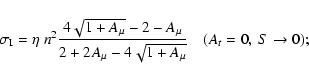
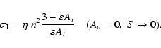
![]() of the unstable modes. In the two limit cases, this equation has solutions for
of the unstable modes. In the two limit cases, this equation has solutions for
![]() at
given
at
given ![]() or
or
![]() ,
which can be easily derived. When At=0, the growth-rate is given by
,
which can be easily derived. When At=0, the growth-rate is given by
We finally turn back to the non-dissipative case, for which we derive the dynamical energy
equation. Introducing the perturbation velocity
![]() ,
and considering only the real part of all variables, we rewrite (A.10) for the stable case p=1 as
,
and considering only the real part of all variables, we rewrite (A.10) for the stable case p=1 as
 |
(A.18) | ||
 |
(A.19) | ||
 |
(A.20) |
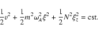
![$\displaystyle {1 \over 2}{\partial \over \partial t} \left[v_\varpi^2 + v_\varp...
...hi \over \partial t} {\partial \xi_\varpi \over \partial \varphi} \right] \cdot$](/articles/aa/full/2007/40/aa7653-07/img236.gif) |
(A.21) |
![$\displaystyle (\sigma^2 - \omega_A^2)~ ( \sigma^2 - \omega_A^2 [1+A ]) + (p-1) ...
...m} \omega_A^2 \right) \left(2 \Omega \sigma+ 2{\omega_A^2 \over m} \right) =0 .$](/articles/aa/full/2007/40/aa7653-07/img32.gif)
![\begin{displaymath}\zeta = -2 \pm m ~ \sqrt{1+A} \quad \hbox{or} \quad
\sigma= {...
...ega} \left[-{1 \over m} \pm {\sqrt{1+A} \over 2} \right] \cdot
\end{displaymath}](/articles/aa/full/2007/40/aa7653-07/img48.gif)

![\begin{displaymath}[A_\mu~ S(A_\mu)]~ \omega_A^4 = 2 \Omega \eta l^2 N_\mu^2 .
\end{displaymath}](/articles/aa/full/2007/40/aa7653-07/img82.gif)
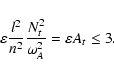
![\begin{displaymath}{l^2 \over n^2} \left[ \varepsilon {N_t^2 \over \omega_A^2} +{N_\mu^2 \over \omega_A^2}\right] = A^*
\end{displaymath}](/articles/aa/full/2007/40/aa7653-07/img97.gif)
![\begin{displaymath}[A^*~ S(A^*) ]~ \omega_A^4 = 2 \Omega \eta l^2 \left[\varepsilon N_t^2 + N_\mu^2 \right] ,
\end{displaymath}](/articles/aa/full/2007/40/aa7653-07/img99.gif)

![$\displaystyle l {P' \over \rho} + \left[-\sigma^2 + {m^2\omega_A^2 \over 1+i \eta s^2/ \sigma} \right] \xi_\varpi$](/articles/aa/full/2007/40/aa7653-07/img201.gif)
![$\displaystyle +\left[- {(l\varpi)m \omega_A^2 \over 1+i \eta s^2 /\sigma} +
{\r...
...ver 1+i \eta s^2 /\sigma} + 2 {\rm i} \Omega \sigma \right] \xi_\varphi
= 0 ~ ,$](/articles/aa/full/2007/40/aa7653-07/img202.gif)
![$\displaystyle {m \over \varpi} {P' \over \rho} - \left[ {\rm i} {(p+1)m \omega_...
...ma} + 2 {\rm i} \Omega \sigma \right] \xi_\varpi - \sigma^2 \xi_\varphi = 0 ~ ,$](/articles/aa/full/2007/40/aa7653-07/img203.gif)
![$\displaystyle +\left[-\sigma^2 + {m^2\omega_A^2 \over 1+{\rm i} \eta s^2/ \sigm...
...amma\sigma} + {N_\mu^2 \over 1+{\rm i} \lambda s^2 / \sigma}\right] \xi_z = 0 ,$](/articles/aa/full/2007/40/aa7653-07/img205.gif)