A&A 473, 357-368 (2007)
DOI: 10.1051/0004-6361:20077412

Quark-nova remnants

I. The leftover debris with applications to SGRs, AXPs, and XDINs

R. Ouyed - D. Leahy - B. Niebergal

Department of Physics and Astronomy, University of Calgary, 2500 University Drive NW, Calgary, Alberta, T2N 1N4, Canada

Received 5 March 2007 / Accepted 24 July 2007

Abstract
We explore the formation and evolution of debris ejected around quark stars in the Quark Nova scenario, and the application to Soft Gamma-ray Repeaters (SGRs) and Anomolous X-ray Pulsars (AXPs). If an isolated neutron star explodes as a Quark Nova, an iron-rich shell of degenerate matter forms from its crust. This model can account for many of the observed features of SGRs and AXPs such as: (i) the two types of bursts (giant and regular); (ii) the spin-up and spin-down episodes during and following the bursts with associated increases in $\dot{P}$; (iii) the energetics of the boxing day burst, SGR1806+20; (iv) the presence of an iron line as observed in SGR1900+14; (v) the correlation between the far-infrared and the X-ray fluxes during the bursting episode and the quiescent phase; (vi) the hard X-ray component observed in SGRs during the giant bursts, and (vii) the discrepancy between the ages of SGRs/AXPs and their supernova remnants. We also find a natural evolutionary relationship between SGRs and AXPs in our model which predicts that the youngest SGRs/AXPs are the most likely to exhibit strong bursting. Many features of X-ray Dim Isolated Neutron stars (XDINs) are also accounted for in our model such as, (i) the two-component blackbody spectra; (ii) the absorption lines around 300 eV; and (iii) the excess optical emission.

Key words: dense matter - accretion, accretion disks - stars: pulsars: general - X-rays: bursts - elementary particles

1 Introduction

Soft $\gamma$-ray Repeaters (SGRs) are sources of recurrent, short ( $t \sim 0.1~{\rm s}$), intense ( $L \sim 10^{44}~\rm {ergs}$) bursts of $\gamma$-ray emission with a soft energy spectrum. The normal patterns of SGRs are intense activity periods which can last weeks or months, separated by quiescent phases lasting years or decades. The three most intense SGR bursts ever recorded were the 5 March 1979 giant flare of SGR 0526-66 (Mazets et al. 1979), the similar 28 August 1998 giant flare of SGR 1900+14 and the 27 December 2004 burst (SGR 1806-20). AXPs are similar in nature but with a somewhat weaker intensities and no recurrent bursting. Several SGRs/AXPs have been found to be X-ray pulsars with unusually high spin-down rates of $\dot{P} / P \sim 10^{-10}$ s^-1, usually attributed to magnetic braking caused by a super-strong magnetic field.

Occasionally SGRs enter into active episodes producing many short X-ray bursts; extremely rarely (about once per 50 years per source), SGRs emit giant flares, events with total energies at least 1000 times higher than their typical bursts. Current theory explains this energy release as the result of a catastrophic reconfiguration of a magnetar's magnetic field. Magnetars are neutron stars whose X-ray emission are powered by ultrastrong magnetic fields, $B \sim 10^{15}$ G. Although the magnetar model has had successes, in this paper we present an alternative model which addresses outstanding questions.

We explore these issues within the quark-nova (QN) scenario (Ouyed et al. 2002; Ouyed et al. 2004; Keranen et al. 2005). In our previous studies we have suggested that CFL (color-flavor locked) quark stars could be responsible for the activity of SGRs and AXPs (Ouyed et al. 2005; Niebergal et al. 2006), and in this paper we extend the QN model by studying in more details the evolution of the QN ejecta (as first discussed in Keränen & Ouyed 2003).

Following the QN explosion we show that a high metalicity shell can form from the neutron star crust. If this matter gains sufficient angular momentum from the central quark star it can form a torus-like structure via the propeller mechanism, which is discussed in the second paper in this series (Ouyed et al. 2006; hereafter refered to as Paper II). However if it does not, as we discuss in this paper, there is instead a thin corotating shell suspended by the quark star's magnetic field pressure. Because the quark star is in a superconducting state it's magnetic field decay is coupled to its period in a manner prescribed by Niebergal et al. (2006), such that as the field decays the shell will drift closer to the star. This movement will shift sections of the shell above the line of neutrality, loosely defined as the polar angle (measured from the equator) above which the magnetic field vector is sufficiently parallel to the gravity vector to allow material to break off from the shell, and fall into the star. Upon collision with the star the pieces of the shell are instantly converted to CFL quark matter (described by Lugones & Horvath 2002), where excess energy is released as high-energy radiation (Ouyed et al. 2004). We propose this as the mechanism responsible for SGR and AXP bursting activity, and also show that SGRs and AXPs differ primarily by age. Another class of objects are also explored, namely X-ray Dim Isolated Neutron stars (XDINs; e.g. Haberl 2004), and we find that these may have evolved from SGRs/AXPs.

This paper is presented as follows. In Sect. 2 we review the concepts of a quark-nova and the expansion/evolution of the ejected material into a shell. Section 3 contains discussions on the geometry of the resulting shell and its self-similar behaviour in time, leading to pieces of the shell breaking off. The subsequent high-energy bursting from these pieces falling into the quark star is then described in Sect. 4, along with methods for estimating the age of SGRs/AXPs. In Sect. 5 the quiescent phase of SGRs/AXPs is discussed in the context of our model, where a simple relation between luminosity and spin-down rate is derived. The changes in period and period derivative observed during bursts are then discussed within the framework of our model in Sect. 6. Section 7 contains case studies for specific SGRs (1806-20 and 1900+14), along with explanations for the presence of an iron line during bursts, correlated X-ray to infrared flux ratio, and the hard spectrum seen in giant flares. We then summarize in Sect. 7.5 some outstanding issues in the current understanding of SGRs/AXPs, and show how our model can provide explanations. Finally in Sect. 8, we discuss XDINs and show how many features are readily explained using our model. We then conclude in Sect. 9.

  
2 Quark nova

In the quark-nova (QN) scenario, the core of a neutron star (NS) shrinks to a stable, compact, quark object before the conversion of the entire star to (u, d, s) matter. By contracting, and physically separating from the overlaying material (hadronic envelope which is mostly made of crust material), the core drives the collapse (free-fall) of the overlaying matter leading to both gravitational and phase transition energy release as high as 10⁵³ ergs in the form of neutrinos. The result is a quark star in the Color-Flavor Locked (CFL) superconducting phase, surrounded by an ejected shell. Although it has been shown that pure CFL matter is rigorously electrically neutral (Rajagopal & Wilczek 2001), other work (Usov 2004, and references therein) indicates that a thin crust is allowed around a quark star due to surface depletion of strange quarks. In our model we have assumed no depletion of strange quarks, which implies a bare quark star.

In the CFL phase there are a total of nine combinations between the gluons and the photon with eight of these combinations subject to the Meissner effect. The only one that does not suffer the Meissner effect involves a combination of electromagnetism and a U(1) subgroup of the color interactions (e.g. Ferrer et al. 2005). In other words the magnetic field will penetrate some phases of the color field but not others. Unfortunately, the relevant calculations are done in effective models of QCD which cannot accurately handle the details of the mixing and the corresponding back reaction of the quarks. Assumptions had to be made (e.g. Meissner effect) in order to proceed with our astrophysical model which implies that we are ignoring the one component that penetrates the superconductor. In the CFL quark star, given our basic assumptions, the magnetic field is contained in the vortex array so the internal field is uniform and equal to the surface field.

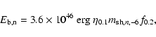
The QN ejecta consists mainly of the neutron star's metal-rich outer layers heated by neutrino bursts. It was shown that up to $10^{-2}~ M_{\odot}$ can be released during the QN (Keränen et al. 2005). Thus our model proposes a high density, metal-rich ejecta surrounding a superconducting quark star.

Within our model there are four possible scenarios as to the outcome of the ejecta. First, if the ejecta is very light then it will become gravitationally unbound from the quark star, where the r-process begins creating heavier elements (Jaikumar et al. 2006). Second, if the ejecta is too heavy it will fall back into the quark star releasing tremendous amounts of energy. This we propose could lead to explosive events reminiscent of short gamma-ray bursts, which we are currently exploring. Third, is the case where the ejecta mass is such that it can be suspended above the surface by the quark star's magnetic pressure. Fourth, the ejecta was formed with enough angular momentum to move into a Keplerian orbit. The third case is discussed in this paper, whereas the fourth is discussed in the second paper of this series.

2.1 Expansion of the ejecta

We consider the dynamics of the shell (of mass $m_{\rm sh}$) ejected during the QN. If the shell's outward momentum is not too large, the interplay between gravity and the QS's magnetic field is dominant. Thus, as the highly conducting shell expands spherically outwards, an electromotive ( $\vec{J}\times\vec{B}$) force is induced to oppose its motion, causing it to continuously decelerate. The natural oscillatory motion created by the magnetic pressure gradient and gravity is resultingly damped out, resulting in the ejecta finding an equilibrium radius where the forces due to the magnetic pressure gradient and gravity are in balance. This equilibrium radius is then given by,

$$R_{\rm m} \simeq 10\ {\rm km}\sqrt{\sin\theta_{\rm B}}\ \frac... ...{\rm QS, 10}^3} {\sqrt{m_{\rm sh, -6} M_{\rm QS, 1.4}}} \cdot$$ (1)

Here we have used $B_{\rm m} = B_{\rm s} (R_{\rm s}/R_{\rm m})^3$ for a dipole magnetic field with a strength at the surface of, $B_{\rm s, 15}$, in units of $10^{15}~\rm {G}$. The star's mass and radius are in units of $1.4 ~M_{\odot}$ and $10~\rm {km}$ respectively, while the mass of the shell, $m_{\rm sh, -6}$, is in units of $10^{-6}~ M_{\odot}$. The line of neutrality, $\theta_{\rm B}$, is measured from the equator and defines the angle above which the gravity vector is no longer mostly perpendicular to the magnetic field vector. If sections of the shell are above this line, they are free to break off and fall into the star's poles along the field lines. The condition for the shell to exist is that it is off the surface of the quark star, $R_{\rm m} > R_{\rm QS}$, which implies $B_{\rm s, 15}^2 R_{\rm QS, 10}^4 \sin\theta_{\rm B} > (m_{\rm sh, -6} M_{\rm QS,1.4})$.

For this equilibrium situation to be achieved the mass and initial velocity of the shell are confined to a somewhat narrow range of values. Although the mass of the shell is self-consistent with previous studies of neutron star crust masses (discussed below), the initial velocity is not similarly constrained. As such, we assume it can take on a range of values, with the small initial velocity case corresponding to the work presented in this paper, and the high velocity case is left for the second paper in this series. We feel that this dichotomy is physical, and explains some observed AXP features well.

Recent work studying natural mechanism of magnetic field amplification in quark matter (just before or during the onset of superconductivity; Iwazaki 2005), shows that 10¹⁵ G magnetic fields are readily achievable. This amplification can occur in quark matter due to the response of quarks to the spontaneous magnetization of the gluons. In contrast, for the magnetar model, the sole proposed mechanism for generating 10¹⁵ G fields requires millisecond proto-neutron stars. This seems to be challenged by recent observations (Allen & Hovarth 2006).

Thus, Eq. (1) implies that for magnetic fields in the range of 10¹⁴- $10^{15}~\rm {G}$, the maximum mass of the shell cannot exceed 10^-8- $10^{-6}~ M_{\odot}$. A higher shell mass translates into $R_{\rm m} < R_{\rm QS}$, meaning that the magnetic field is not sufficiently strong to stop the shell from promptly falling back onto the star. This situation is very possible but not considered in this paper, as it is left for future work.

The shell's size is determined by the NS crust density profile (Datta et al. 1995), and is of the order of (0.012- $0.025)]\times R_{\rm QS}$ corresponding to shell masses of the order of (10^-8- $10^{-6})M_{\odot}$ for densities of $(1.8\times 10^{8}$- $5.5\times 10^{10})$ g/cc. We note that if degenerate, the shell will always be in relativistic degeneracy since the densities are above $\rho_{\rm cr} = 7.3\times 10^{6} \mu_{\rm e}$ g/cc (Lang 1974). Here, $\mu_{\rm e}$ is the mean mass per electron and is taken to be $\mu_{\rm e}\approx 2$ since the shell's maximum density is below the neutron drip density, $\sim$ $4\times 10^{11}$ g cm^-3 .

The transition from Fermi-Dirac to Boltzmann statistics occurs at the degeneracy temperature $T_{\rm fermi} \simeq 76.2~\rm {MeV}~\rho_{\rm 10}^{2/3}$for a non-relativistic gas and $T_{\rm fermi} \simeq 8.8~\rm {MeV}~\rho_{\rm 10}^{1/3}$ for a relativistic gas (e.g. Lang, p. 253). So, for the shell to be born degenerate at 10 MeV, it implies a minimum density of $\sim$10¹⁰ g/cc which translates to an ejected mass of $\sim$ $10^{-7}~M_{\odot}$. We note that even if the shell density at birth is less than $\sim$10¹⁰ g/cc, (blackbody) cooling during the expansion of the ejecta to $R_{\rm m}$ results in a shell temperature of less than 1 MeV, thus, yielding a degenerate shell.

Once the shell reaches the magnetic radius $R_{\rm m}$, it will have expanded to a thickness of, $\Delta R_{\rm m}$, such that it satisfies hydrostatic equilibrium. Using the relativistic degenerate equation-of-state ( $P = \varkappa\rho^{4/3}$ where $\varkappa = 1.244\times 10^{15} \mu_{\rm e}^{-4/3}$), the width of the shell, positioned at $R_{\rm m}$, can be calculated to be,

$$\frac{\Delta R_{\rm m}}{R_{\rm m}} = 2.1\times 10^{-2} m_{\rm shell, -6}^{1/4} M_{\rm QS, 1.4}^{-3/4} .$$ (2)

This implies that the shell's thickness does not change much when it reaches $R_{\rm m}$. The corresponding average density of the shell at the magnetic radius is then,

$$\rho_{\rm m} = 7.58\times 10^{9}~{\rm g/cc}\ m_{\rm sh, -6}... ...} M_{\rm QS, 1.4}^{9/4} B_{\rm s, 15}^{3} R_{\rm QS, 10}^9 ,$$ (3)

implying that the shell is relativistic degenerate.

2.2 Energy release

The internal energy of the expanding ejecta is $U = N (3/5)\epsilon_{\rm F} \left[1 + \frac{5\pi^2}{12}\left(\frac{kT}{\epsilon_{\rm F}}\right)^2\right]$where $N= m_{\rm shell}/\mu_{\rm e} m_{\rm H}$, is the total number of electrons. The Fermi energy in this case is $\epsilon_{\rm F} \sim 8.8\ {\rm MeV} \rho_{10}^{1/3}$ (e.g. Pathria pg. 200). As a result of the heating of the electrons, the optically thick shell will radiate approximately as a blackbody,

$$L_{\rm sh} = 4\pi R_{\rm sh}^2 \sigma T_{\rm sh}^4 .$$ (4)

The total energy it releases as it relocates to $R_{\rm m}$ is then (taking $kT \ll \epsilon_{\rm F}$)

$$\Delta U_{\rm F} \sim 5.2\times 10^{45}~{\rm erg} \ m_{\rm sh... ... \left(\rho_{\rm i,10}^{1/3} - \rho_{\rm m,10}^{1/3}\right) ,$$ (5)

where $\rho_{\rm i,10}$ and $\rho_{\rm m,10}$ are the densities of the shell initially and at magnetic equilibrium radius respectively, in units of $10^{10}~\rm {g/cc}$. This energy released during expansion is done so in roughly a millisecond.

We have not investigated the fate of this energy release, whether it is absorbed by adiabatic expansion losses or radiated. What is crucial to our model is the fact that the shell remains degenerate at $R_{\rm m}$ which is guaranteed by hydrostatic equilibrium.

2.3 Angular momentum transfer

For a magnetic radius, $R_{\rm m}$, larger than the corotation radius the propeller will take effect (Schwartzman 1970; Illarionov & Sunyaev 1975), deflecting the QN shell into a torus on the equatorial plane. Using an angular momentum conservation argument, we can estimate the location of such a torus by writing

$$R_{\rm m}^2 \Omega_{\rm QS} = R_{\rm t}^2 \Omega_{\rm K} ,$$ (6)

where $R_{\rm t}$ is the equatorial location of the torus in a Keplerian orbit around the quark star, and $\Omega_{\rm K} = \sqrt{GM_{\rm QS}/R_{\rm t}^3}$ is the Kepler rotation. Applying Eq. (1) implies a torus radius of,

$$R_{\rm t} = \frac{R_{\rm m}^4 \Omega_{\rm QS}^2}{G M_{\rm Q... ... { m_{\rm sh, -6}^{2} M_{\rm QS, 1.4}^3 P_{{\rm i,ms}}^{2}} ,$$ (7)

where the birth period, $P_{\rm {i,ms}}$, is given in units of milliseconds.

However, in order to actually form a torus we require enough angular momentum transfer to guarantee $R_{\rm t} > R_{\rm m}$. This translates into an upper limit on the initial period of,

$$P_{\rm {i,lim}} < 0.46~{\rm ms}~ \frac{\left(\sin\theta_{\rm ... ...}^{9/2} } {m_{\rm {sh,}-6}^{3/4} M_{\rm {QS,}1.4}^{5/4}} \cdot$$ (8)

This presents two cases: we study the first in this first paper when the star's initial period is too large for torus formation. This is where the shell will remain at $R_{\rm m}$ and be in corotation with the magnetosphere. The second case where the shell can achieve a Keplerian orbit and form a torus is studied in Paper II (Ouyed et al. 2006).

  
3 Co-rotating degenerate shell

3.1 Shell geometry

The area of a shell at the magnetic equilibrium radius, $R_{\rm m}$, is $A_{\rm sh} = 4\pi R_{\rm m}^2 \sin\theta_{\rm B}$, where $\theta_{\rm B}$ is the polar angle (measured from the equator) and defines the line of neutrality. In other words, for $\theta > \theta_{\rm B}$ the shell material is free to "slip'' along the magnetic field lines onto the star, whereas for $\theta < \theta_{\rm B}$ the shell material is suspended by magnetic pressure. Thus, the geometry is such that there is a thin shell at the equator subtending an angle of $2\theta_{\rm B}$, and empty regions at the poles. The shell is shaped in the star's distorted magnetic dipole with an inward bulge at the equator, and the radius of the shell at the equator, under hydrostatic balance, can be shown to be roughly half that at $\theta_{\rm B}$.

  
3.2 Self-similarity: shell dynamics and evolution

The radius of the shell, $R_{\rm m}$, is proportional to the magnetic field strength (i.e. Eq. (1)), so we use the magnetic field decay prescribed by Niebergal et al. (2006) to calculate the radius in time. This is because the quark star itself is in the superconducting phase, implying that vortex expulsion couples field decay and period evolution.

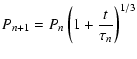
After a characteristic time, $\tau_{n}$ (as defined by Eq. (4) in Niebergal et al. 2006), the shell will respond to the decaying field by moving towards the star, resulting in a new equilibrium radius. During this movement, sections of the shell will be shifted above the line of neutrality, $\theta_{\rm B}$, where they will be broken off and fall into the star along the magnetic field lines. Upon colliding with the quark star these shell pieces will be converted immediately to CFL quark matter, releasing excess energy in the form of radiation, which in our model is an SGR/AXP burst. We then have a new state, n+1, where the shell has moved towards the star, lost mass, and is now sitting at radius $R_{{\rm m}, n+1}$ with a mass  $m_{{\rm sh}, n+1}$.

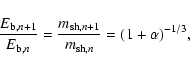
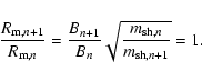
The new characteristic decay time, period of rotation, period derivative, and magnetic field are respectively,

    

$$\tau_{n+1} = \kappa \frac{P_{n+1}^2}{B_{n+1}^2}$$ (9)

$$P_{n+1} = P_{n} \left(1+\frac{t}{\tau_{n}}\right)^{1/3}$$ (10)

$$\dot{P}_{n+1} = \frac{P_{n}}{3\tau_{\rm n}} \left (1+\frac{t}{\tau_{n}}\right)^{-2/3}$$ (11)

$$B_{n+1} = B_{n} \left(1+\frac{t}{\tau_{n}}\right)^{-1/6} ,$$ (12)

where the constant $\kappa = 8.8\times 10^{38}~\rm {G}^2~\rm {s}^{-1}$, is for a quark star with a mass of $1.4 ~M_{\odot}$ and radius of $10~\rm {km}$. Also, t, is the time elapsed since the previous burst (or birth of the quark star if it is the case). Taking the ratio of the new characteristic time to the old gives,

$$\frac{\tau_{n+1}}{\tau_n} = 1 + \frac{t}{\tau_n} = 1+ \alpha ,$$ (13)

where $\alpha \equiv t/\tau_n$ defines the typical decay time of the magnetic field for each epoch n. Because of the self-similar nature of the problem, $\alpha$is roughly constant from one epoch to another, which implies that the time interval between two successive bursts,

$$\Delta t_{n+1} = \alpha \tau_{n+1} = \alpha (1+\alpha)^{n}\tau_{n} ,$$ (14)

increases in time on average.

So after a time $t= \alpha \tau_{n}$, the magnetic field decays and the shell originally sitting at $R_{{\rm m},n}$ moves in closer to the star. Now by keeping the mass of the shell constant as it slowly drifts in from $R_{\rm m}$ to an inner radius $R_{\rm in}$ and applying Eq. (1) we can write,

$$R_{\rm in}/R_{\rm m} = B_{n+1}/B_{n} = (1+\alpha)^{-1/6} .$$ (15)

In the above equation the notation used implies that the shell reaches $R_{\rm in}$ when the surface magnetic field has decayed to B_n+1. Following this, the shell will then suddenly lose mass at $R_{\rm in}$, due to the pieces of the shell closest to the poles being shifted above the line of neutrality, $\theta_{\rm B}$, and breaking off. The resulting change of mass of the shell can be realized by considering the area of shell material below the line of neutrality while keeping density in the shell roughly constant during the process,

$$\frac{m_{{\rm sh,}n+1}}{m_{{\rm sh,}n}} = \frac{4\pi \sin\th... ... = \frac{R_{\rm in}^2}{R_{{\rm m}, n}^2} = (1+\alpha)^{-1/3} .$$ (16)

The shell will now be less massive causing it to rapidly (i.e. keeping B constant, $B_{n+1}= B_{\rm in}$) equilibriate by moving further away from the star to a new radius that defines the (n+1) state. It so happens, this new radius is the same as the original. This is seen from Eq. (1),

$$\frac{R_{{\rm m,} n+1}}{R_{{\rm m,}n}} = \frac{B_{n+1}}{B_{n}} \sqrt{\frac{m_{{\rm sh,}n}}{m_{{\rm sh,}n+1}}} = 1 .$$ (17)

Therefore as the shell adjusts over time, it stays at roughly the original radius $R_{{\rm m},n}$. In other words, it oscillates about the same position while losing mass. This mass loss can be determined appealing to Eqs. (15), (16),

$$\Delta m_{{\rm sh,}n} = m_{{\rm sh}, n} - m_{{\rm sh}, n+1}= f\left(\alpha\right) \times m_{{\rm sh},n} ,$$ (18)

where we define $f(\alpha)$ as,

$$f\left(\alpha\right) = \left(1-\left(1+\alpha\right)^{-1/3}\right) .$$ (19)

Thus, the amount of mass lost during a burst in this self-similar model (Eq. (18)) is determined by $\alpha$. The corresponding energy release is,

 

$$E_{{\rm b},n} \eta \Delta m_{{\rm sh,}n} c^2 = \eta m_{{\rm sh,}n}c^2 f\left(\alpha\right)$$ = (20)

$$1.8\times 10^{47} \ {\rm erg}\ \eta_{0.1} m_{\rm {sh,}-6} f(\alpha) \ ,$$ =

where $\eta_{0.1}$ is the energy conversion efficiency factor taken to be $\sim$0.1. We also note that the ratio between succesive burst energies is,

$$\frac{E_{{\rm b}, n+1}}{E_{{\rm b}, n}} = \frac{m_{{\rm sh}, n+1}}{m_{{\rm sh}, n}} = (1+\alpha)^{-1/3} ,$$ (21)

which implies that the bursts weaken in time. This is expected since the shell's mass is decreasing in time.

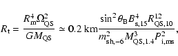
In our model, AXPs are merely older versions of SGRs, thus one would expect SGR bursts to be more intense and frequent. As can be seen in Table 1 (where the objects are in order of decreasing estimated age), there is seemingly a decreasing trend in burst intensity and frequency as one moves from younger to older objects. It may be that both types of bursts have this trend, however, we do not feel there is enough events to draw any conclusions. This is a potential test for our model.

  
4 The bursting phase

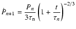
The magnetic energy due to field decay is released continuously over a long timescale (thousands of years) and gives the steady x-ray luminosity of SGRs and AXPs (see Sect. 5). What is important and unique about the shell (i.e. the accretion energy) is that the energy is released in bursts, and the shell sitting at $R_{\rm m}$ offers a natural mechanism/torque for sudden changes in period derivative.

After time $t\sim \alpha \tau$, the magnetic field decays substantially and the entire shell moves in to $R_{\rm in}/R_{\rm m}\sim (1+\alpha)^{-1/6}$. A larger $\alpha$ means the shell moves closer to the star, causing larger sections to be shifted above the line of neutrality, implying larger bursts.

Another possible scenario is that giant bursts are due to global instabilities like Rayleigh-Taylor while regular bursts are due to chunks breaking-off the edge of the shell. We assume that the Rayleigh-Taylor instability does not act due to the long timescale for magnetic penetration of the conducting shell (see Sect. 4.1 in Paper II). What is presented below is intended to present the overall scenario and follow-up work (i.e. numerical simulations) is necessary to investigate the effects global instabilities might have on this simplified picture.

4.1 Giant bursts: $\alpha$ $\simeq$ 1

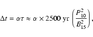
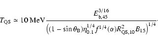
If the time needed for the shell to move in sufficiently to have pieces broken off is roughly equal to the characteristic field decay time, then $\alpha=1$, and $\sim$20% of the shell's mass is lost during the burst. According to Eq. (20), the corresponding energy release is,

$$E_{\rm {b},n} = 3.6\times 10^{46} \ {\rm erg}\ \eta_{0.1} m_{{{\rm sh},n,}-6} f_{0.2} ,$$ (22)

where $f_{0.2} = f(\alpha =1)$ and $m_{{{\rm sh},n,}-6}$ is the current mass of the shell in units of $10^{-6}~ M_{\odot}$. The waiting time between each bursts is on average,

$$\Delta t = \alpha \tau \approx \alpha\times 2500~{\rm yr}\ \left(\frac{P_{10}^2}{B_{15}^2}\right) ,$$ (23)

where P₁₀ is the spin period in units of $10~\rm {s}$, and the magnetic field is in units of $10^{15}~\rm {G}$. One can see here that, because B decreases and P increases in time, the waiting times are increasingly less frequent as the object ages. Given the range in B derived for SGRs in our model (see Table 1), this implies a burst frequency of $\simeq$ $1/(\alpha 1000\ {\rm yr})$ per object.

Figure 1: The upper panel is a P-$\dot{P}$ diagram with SGRs/AXPs and XDINSs plotted. The solid curve is a plot of Eq. (26) with a burst energy of $E_{\rm b}= 10^{46}$ erg, $\alpha = 2$, and $R_{\rm m}= 20$ km. Also shown are curves for $R_{\rm m}=100$ km, $\alpha = 2$ and energies $E_{\rm b}= 10^{44}$ erg s-1 (dotted) and $E_{\rm b}= 10^{41}$ erg s-1 (dashed). These line of constant energy move leftwards as an object ages. In the lower panel luminosity is plotted against period derivative according to Eq. (30). The upper and lower solid lines represent a magnetic to X-ray conversion efficiency, $\eta _{\rm X}$, of 1 and 0.01 respectively, and the dashed line is the luminosity averaged over all viewing angles (for $\eta _{\rm X}=1$). Since $\dot{P}\propto 1/\rm{age}$, objects further to the left are generally older.

Open with DEXTER

   
4.2 Regular bursts: $\alpha$ $\ll$ 1

If pieces of the shell are able to break off as the shell moves in by only a small amount, then $\alpha \ll 1$. This corresponds to small pieces of the shell falling into the star and, in our model, leads to regular-sized bursts. This process can be interpreted as small oscillations around $R_{\rm m}$ consistent with small fractional mass-loss episodes by the shell. Observationaly, regular bursts are known to follow a power-law distribution in energies which in our model would be due to a power-law distribution in $\alpha$. Clearly, the detailed mechanism which determines $\alpha$ would be different for giant bursts and regular bursts, and would require numerical simulations to understand.

For $\alpha \ll 1$, Eq. (18) approximates to $\Delta m_{{\rm sh,}n} \simeq (\alpha/3) m_{{\rm sh,}n}$ which yields burst energies of,

$$E_{\rm b} \sim \alpha\times \left( 6\times 10^{46}\ {\rm erg~s}^{-1}\right)~ \eta_{0.1} m_{{\rm s},n,-6} .$$ (24)

For $\alpha = 10^{-6}$, a burst energy of $E_{\rm b}\sim 6\times 10^{40}$ erg is attained, and one should expect a waiting time of $\Delta t \sim 1$ day (see Eq. (23)), for a star with a $7~\rm {s}$ rotation period and field strength of $10^{15}~\rm {G}$.

Thus, in our model the difference between regular and giant bursts is due to the size of piece that breaks off the shell. Although the size is of a stochastic nature, we expect younger objects (i.e. the SGRs) to have a more unstable shell, resulting in more large pieces breaking off, causing more frequent and intense bursts. For older objects (i.e. the AXPs) the shell becomes more stable with age resulting in weaker, less frequent, bursts.

4.3 The P - $\dot{P}$ diagram

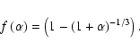
From Eqs. (10) and (12), the magnetic field is related to the period and period derivative by,

$$B = \sqrt{3 \kappa P\dot{P}} .$$ (25)

Furthermore, combining this and the equation for $R_{\rm m}$ (Eq. (1)) with Eq. (20) one can show that,

$$P \dot{P}_{-11} \simeq 21 \frac{R_{\rm m,10}^2}{\sin\theta_{\... ...s \frac{E_{\rm b, 47}}{\eta_{0.1} f\left(\alpha\right)} \cdot$$ (26)

Illustrated in the upper panel of Fig. 1, are cases with large and small $\alpha$. The solid curve is for $E_{\rm b}= 10^{46}$ erg s^-1, $\alpha = 2$, and $R_{\rm m}= 20$ km, and fits well with the boxing day event. Also shown are two curves for $R_{\rm m}=100$ km, $\alpha = 2$ and energies $E_{\rm b}= 10^{44}$ erg s^-1 (dotted) and $E_{\rm b}= 10^{41}$ erg s^-1 (dashed). The lines of constant burst energies in the upper panel of Fig. 1 move to the left as time increases (as the object ages). This can be seen from Eq. (21) in Sect. 3.2 which shows the burst energy decreasing in time. We also note that as objects evolve further to the left, the bursts are weaker and less frequent, which is why AXPs in our model evolve from SGRs.

  
4.4 Age estimate

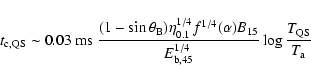
To determine the exact age of AXPs/SGRs in our model, one would need to know the entire bursting history of the object which is impossible. For a real situation the burst sizes are variable implying a different $\alpha$ for each burst. So to approximate the age in the simplest case (when $\alpha$ is constant over time on average), the age elapsed since the QN is,

$$t_{\rm QN} = \sum_{i=1}^{n} \alpha \tau_{i} .$$ (27)

Using Eq. (13) the series can be summed to yield

$$t_{\rm QN} = \tau_{n} \left( 1 - (1+\alpha)^{-n}\right) .$$ (28)

Provided that there has been a large number of bursts ($n\gg1$),

$$\tau_{n}=P_{n}/3\dot{P}_{n}$$ (29)

is a good estimate of the age, however we do expect $\alpha$ to vary from one burst to another. Although for SGRs, the energy in the large bursts ( $\alpha\sim 1$) dominates the small bursts ( $\alpha\sim 10^{-6}$), resulting in an age very close to that of Eq. (28). This age also happens to be the age estimate derived from Eqs. (9)-(11) when assuming $t\gg\tau$, which is reasonble for AXPs in our model. So our model predicts the age of $\sim$ $0.5 P/3\dot{P}$ for SGRs, and $\sim$ $P/3\dot{P}$ for AXPs and XDINSs. However, without knowing the burst history we cannot derive the initial period and magnetic field (see Eqs. (10) and (12)).

One may be tempted to use the age of the associated parent supernova remnant to estime the age of the SGR/AXP, but in our model these ages are neccesarily different. This is due to the time required for a neutron star to reach quark deconfinement densities (Staff et al. 2006), as well as the time needed for strange quark nucleation (i.e. u,d to u,d,s) to occur (Bombaci et al. 2004). Together these delays can easily add up to the age difference between SGRs/AXPs and their supernova remnants.

  
5 The quiescent phase

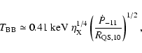
The X-ray luminosity during the quiescent phase of SGRs/AXPs in our model is due to vortex expulsion from spin-down. The magnetic field contained within the vortices is also expelled, and the subsequent magnetic reconnection leads to the production of X-rays. From Eq. (22) in Ouyed et al. (2004) and Eqs. (10)-(12), the luminosty emitted from this process is,

$$L_{\rm X} \simeq 2.01\times 10^{35}\ {\rm erg s}^{-1} \eta_{\rm X} \dot{P}_{-11}^2 ,$$ (30)

where $\eta _{\rm X}$ is the efficiency parameter inherent in the conversion from magnetic energy to radiation. The lower panel in Fig. 1 shows our model of luminosty versus period derivative as compared to the quiescent X-ray luminosities of AXPs, SGRs and XDINSs.

The scatter in the AXPs/SGRs data can be explained within our model by considerations of shell geometry and viewing angle. More specifically, any X-rays being emitted from the star's surface towards the solid angle filled by the shell ( $4\pi\sin\theta_{\rm B}$) will be affected due to absorption by the shell. X-rays are then able to escape from an open area at the poles with a solid angle on the order of $\left(4\pi (1-\sin\theta_{\rm B})\right)$. Because we statistically observe viewing angles equally from all directions, this would imply an average (geometrical mean) lumimosity of $L_{\rm X}\times (1-\sin\theta_{\rm B}) \sim 2.7\times 10^{34}\eta_{\rm X}\dot{P}_{-11}\ {\rm erg~s}^{-1}$, assuming $\theta_{\rm B}=60^{\circ}$. This is plotted by the dotted line in the lower panel of Fig. 1. Thus, the scatter in data is a combination of X-ray production efficiency and viewing angle effects. The two "outliers'' namely, AXP 1E2259+586 and AXP 4U0142+615 can be explained as those AXPs/SGRs born in the propeller regime so that they are surrounded by a degenerate torus instead of a shell, and are discussed in more detail in Paper II.

  
5.1 The two-component blackbody

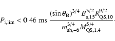
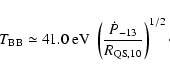
Our model provides an explanation to the two component blackbody spectrum that may be seen in SGRs/AXPs (i.e. Israel 2002). This is realized by considering the blackbody temperature as set by the X-ray continuum luminosity, $L_{\rm X} = 4\pi R_{\rm QS}^2 T_{\rm BB}^4$, to be

$$T_{\rm BB}\simeq 0.41\ {\rm keV}\ \eta_{\rm X}^{1/4} \left(\frac{\dot{P}_{-11}}{R_{\rm QS, 10}}\right)^{1/2} ,$$ (31)

where we made use of Eq. (30) for $L_{\rm X}$ and adopted the fiducial value $R_{\rm QS}=10$ km.

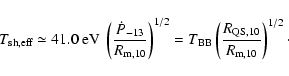
The effective shell temperature in our model is also set by the X-ray continuum luminosity, $L_{\rm X}\sin\theta_{\rm B} = 4\pi R_{\rm m}^2 \sin \theta_{\rm B} \sigma T_{\rm sh,eff}^4$, and is

$$T_{\rm sh,eff} \simeq 0.41 \ {\rm keV}\ \eta_{\rm X}^{1/4}\left(\frac{\dot{P}_{-11}}{R_{\rm m, 10}}\right)^{1/2}\cdot$$ (32)

Thus there is two temperatures from two different emitting blackbodies, namely the quark star and the surrounding shell.

Whether or not the blackbody component from the shell could actually be observed or not hasn't been considered. If it can not, then the magnetic field strengths around CFL quark stars is still at a magnitude that can produce the synchrotron break (i.e. blackbody plus power law) that is usually assumed for SGRs/AXPs. We only assert that if the blackbody emission from the shell could be observed, then its temperature is such that it correlates well with a two-component blackbody spectrum model.

  
6 Period changes and torques

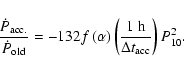
Angular momentum exchange between the shell and the star occurs during the shell's inward and outward movements, and would manifest itself as changes in rotational period and period derivative during bursts. We start with the inward drift where the moment of inertia of the star decreases, causing it to spin-up.

6.1 Inward shell drift: spin-up

In our model the inward shell drift occurs while the vortex (i.e. magnetic flux) expulsion mechanism, as discussed in Niebergal et al. (2006), is coupling the spin period and field decay as described in Eqs. (9)-(12). The spin-up torque from a decreasing moment of inertia occurs slowly during the magnetic field decay timescale over time $\alpha \tau$, and is negligible compared to the spin-down due to vortex expulsion.

The shell eventually reaches an inner radius where it is unstable in the magnetic field geometry, and pieces start to break off above $\theta_{\rm B}$. As the pieces fall in along field lines to the polar regions and collide with the star, angular momentum is transferred. This transfer and the change in moment of inertia, $\Delta I$, as we show below would correspond to a star spinning-up during bursts (i.e. accretion of chunks). The change in moment of inertia from the increase in mass and radius of the star is given by,

$$\frac{\Delta I}{I} = \frac{5}{3}\frac{\Delta m}{M_{\rm QS}} ,$$ (33)

where the accreted matter is converted into CFL matter at the star's density. Taking into account the angular momentum, $\Delta L$, from the infalling (from $R_{\rm m}$) shell material we get,

$$\frac{\Delta P}{P} = \frac{\Delta I}{I} - \frac{\Delta L}{L} ... ...\left(1 - \frac{3}{2}\frac{R_{\rm m}^2}{R_{\rm QS}^2}\right) ,$$ (34)

where a quark star mass and radius of $M_{\rm QS}=1.4~M_{\odot}$ and $R_{\rm QS}=10~\rm {km}$is used, and will be assumed for the remainder of this section. Making use of Eqs. (1) and (18) for $R_{\rm m}$ and $\Delta m$ respectively one arrives at,

$$\frac{\Delta P}{P} \simeq -1.8 \times 10^{-6} f\left(\alpha... ...t(1 - \frac{3}{2}\frac{R_{\rm QS}^2}{R_{\rm m}^2}\right) \cdot$$ (35)

Using Eq. (25), the equation above can be recast into

$$\frac{\Delta P}{P} \simeq - 4.75\times 10^{-7} f(\alpha) P_{10} \dot{P}_{-11} ,$$ (36)

where P₁₀ is the spin period in units of $10~\rm {s}$, $\dot{P}_{-11}$ is the period derivative in units of 10^-11, and we had assumed that $R_{\rm m} \gg R_{\rm QS}$.

If the accretion occurs during a time interval, $\Delta t_{\rm acr}$, the spin-up rate, $\dot{P}_{\rm acc.}= \Delta P/\Delta t_{\rm acc.}$, can be estimated by dividing both sides of Eq. (35) by $\Delta t_{\rm acc.}$. By noting that $\dot{P}_{\rm old} = B^{2}/(3\kappa P)$ we arrive at

$$\frac{\dot{P}_{\rm acc.}}{\dot{P}_{\rm old}} = - 132 f\left(\... ... \left(\frac{1~\rm {h }}{\Delta t_{\rm acc}}\right) P_{10}^2 .$$ (37)

6.2 Outward shell rebound: spin-down

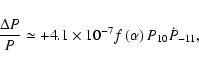
Following the accretion events, during the fast shell rebound, angular momentum is transfered from the star to the shell to keep it co-rotating, resulting in an increase in the spin-down rate of the star. The magnetic coupling between the star and the shell implies that the star will lose angular momentum and spin-down. As the star moves outward from radius $R_{\rm in}$ back to $R_{\rm m}$, conservation of angular momentum of the star/shell system implies $L_{\rm QS, in}+L_{\rm shell, in} = L_{\rm QS, m} + L_{\rm shell, m}$. That is

$$\frac{\Delta P}{P} = + \frac{5}{2}\frac{m_{\rm sh}}{M_{\rm QS... ...^2}{R_{\rm QS}^2} - \frac{R_{\rm in}^2}{R_{\rm QS}^2}\right) ,$$ (38)

or by using Eqs. (1) and (15) one gets,

$$\frac{\Delta P}{P} \simeq + 4.1\times 10^{-7} f\left(\alpha\right) P_{10}\dot{P}_{-11} ,$$ (39)

which as it turns out is insignificant as compared to mass loss from the shell's atmosphere.

  
6.3 Shell atmosphere loss: spin-down

Observationally, an increase in spin-down has been seen to last for $\sim$18 days, as in the case of AXP1E2259, and $\sim$80 days for SGR1900+14. In our model this is readily explained by the heating of the degenerate shell by the burst, and the subsequent release of a portion of it's atmosphere. Because a thin layer on the shell's surface is in the non-degenerate phase, a fraction of it is blown away via the propeller mechanism, removing angular momentum from the system over time.

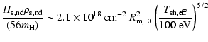
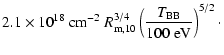
To determine the amount of atmosphere present on the shell during the quiescent phase, we consider the critical density, $\rho_{\rm sh,nd}$, of the shell to ensure degeneracy which is found by setting $T_{\rm sh,eff}= T_{\rm Fermi} \simeq 76.2\ {\rm MeV} \rho_{\rm sh,nd, 10}^{2/3}$, where the density is written in units of $10^{10}~\rm {g/cc}$. So the gas will be non-degenerate below densities of,

$$\rho_{\rm sh,nd} \simeq 3.6\times 10^{3}\ {\rm g/cc}\ \left(\frac{kT_{\rm sh,eff}}{1\ {\rm keV}}\right)^{3/2} \cdot$$ (40)

The scale height of the non-degenerate, upper layers, of the shell can be estimated to be

$$H_{\rm sh,nd} \simeq \frac{k T_{\rm sh,eff}}{(\mu_{\rm Fe} m_... ... m, 10}^2 \left( \frac{T_{\rm sh, eff}}{1 ~{\rm keV}}\right) ,$$ (41)

where $g = GM_{\rm QS}/R_{\rm m}^2\sim 1.87\times 10^{14}/R_{\rm m,10}^2\ {\rm cm~s}^{-2}$ is the effective gravity. Thus, the mass of the non-degenerate portion of the shell is,

 

$$m_{\rm sh,nd} \simeq 4\pi R_{\rm m}^2 \sin\theta_{\rm B} \ H_{\rm sh, nd} \rho_{\rm sh, nd}$$

$$\sim 3.6\times 10^{15} \ {\rm gm.} \ R_{\rm m,10}^4 \left( \frac{kT_{\rm sh, eff}}{1~ {\rm keV}}\right)^{5/2} ,$$ (42)

where $\theta_{\rm B}=60^{\circ}$ was used.

Following a bright burst, with luminosity $L_{\rm b,44}$ (in units of $10^{44}~\rm {erg~s}^{-1}$), the shell gets reheated to temperatures of the order $T_{\rm sh}(t) \simeq 50\ {\rm keV} (L_{\rm b, 44}(t)/R_{\rm m,10})^{1/4}$. The corresponding atmospheric (non-degenerate) mass in terms of the burst energy (in units of $10^{44}~\rm {erg}$), is then

$$m_{\rm sh, nd}(t) \simeq 6.32\times 10^{19}\ {\rm gm.}\ R_{\rm m,10}^{27/8}\ L_{\rm B,44}^{5/8}(t) .$$ (43)

So the trigger mechanism is that the temperature needs to be high enough for the atmosphere to leak away from the shell, most likely in the form of a pressure driven wind. Once it is gravitationally unbound it is kept in co-rotation by the magnetic field out to the light cylinder, providing an efficient propeller. The angular momentum per unit mass lost at the light cylinder is $c^2/\Omega$which gives a new spin-down rate for the quark star of,

$$\dot{P}_{-11,{\rm new}} \simeq 2 \dot{m}_{12} P_{\rm 10}^3 ,$$ (44)

where the estimated mass-loss rate, $\dot{m}_{12}$, is in units of $10^{12}\ {\rm g\ s}^{-1}$.

The change in period due to mass lost at the light cylinder is also written as,

$$\frac{\Delta P}{P} = \frac{5}{2}\frac{\Delta m_{\rm sh, nd}}{M_{\rm QS}} \left(\frac{R_{\rm lc}}{R_{\rm QS}}\right)^2 ,$$ (45)

where $R_{\rm lc}$ is the radius to the light cylinder. Assuming $\Delta m_{\rm sh,nd}= \zeta m_{\rm sh,nd}$ where $\zeta$ is the portion of the non-degenerate atmosphere lost to the light cylinder and $m_{\rm sh, nd}$is the peak of the atmospheric mass during the burst. We get,

$$\frac{\Delta P}{P} = 1.3\times 10^{-4} \ \zeta L_{\rm B,44}^{5/8} P_{10}^2 R_{\rm m,10}^{27/8} ,$$ (46)

where in the equation above we use the peak burst luminosity which we represent by the subscript "B'' as to differentiate it from $L_{\rm b, 44}(t)$ .

Because the shell cools, there is decreasing amounts of matter available to drive the increased spin-down rate. Thus this new rate is temporary and the timescale for it to decay back to the previous rate can be estimated by, $t_{\dot{P}} = \Delta m_{\rm sh,nd}/\dot{m}$, or,

$$t_{\dot{P}} = 4 ~{\rm yrs}\times \zeta L_{\rm B,44}^{5/8} R_{\rm m,10}^{27/8} P_{10}^3 \dot{P}_{-11,{\rm new}}^{-1} .$$ (47)

One should keep in mind that in reality the mass loss rate is decreasing in time. Determining better estimates for this requires knowledge of $\zeta$ which is beyond the scope of this paper.

  
7 Application to SGRs and AXPs

7.1 SGR 1806-20: the boxing day SGR

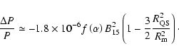
The most recent and brightest giant flare came from SGR 1806-20 on Dec. 27, 2004. This flare lasted about 5 min and had a peak luminosity of about $2 \times 10^{47}\ {\rm erg~s}^{-1}$. For a distance to SGR 1806-20 of 15 kpc, it is estimated that an (isotropic equivalent) energy release of $2 \times 10^{46}$erg occured in the spike, and $5 \times 10^{43}$ erg in the tail.

In our model the energy is readily accounted for. The observed P and $\dot{P}$imply (from Eq. (25)) that $B \sim 1.3\times 10^{15}$ G, which translates to an energy of $3.6\times 10^{46}$ erg for $\alpha=1$ and $R_{\rm m}= 20$ km (see Eq. (20)).

In the year leading up to the SGR 1806-20 giant flare, well-sampled X-ray monitoring observations of the source with the Rossi X-ray Timing Explorer (RXTE) indicated that it was also entering a very active phase, emitting more frequent and intense bursts as well as showing enhanced persistent X-ray emission which was, a prelude to the unprecedented giant flare. In our model, this prelude would correspond to increasing amounts of shell pieces breaking off above $\theta_{\rm B}$ as the shell moves in rapidly closer to the star. This situation is likely only when the quark star's magnetic field is strong such that it is decaying quickly, implying the object is young, which is the case with SGR 1806-20. Furthermore, because $\sim$$20\%$ of the shell's mass was lost in this giant flare, the leftover smaller shell, once re-adjusted to $R_{\rm m}$ following the event, will have less capability to produce flares of the same magnitude as the previous one (see Eq. (21)).

The sharp initial rise of the main spike in the boxing day flare was of the order of 1 ms (Palmer et al. 2005). In our model, a lower limit on the rise time,

$$t_{\rm rise,min } = \frac{\Delta R_{\rm m}}{v_{\rm ff}} ,$$ (48)

is determined by the time it takes a typical chunk of radius $\Delta R_{\rm m}$to cross the star surface, and be converted to CFL quark matter. Larger rise times would correspond to groups of shell pieces accreting simultaneously. To a first approximation we assume that the shell piece crosses the quark star surface at maximum (free-fall) velocity of, $v_{\rm ff}= \sqrt{GM_{\rm QS}/R_{QS}}$. Making use of Eqs. (2), (20) and (25) we get,

$$t_{\rm rise, g} > 0.5~\mu {\rm s} \ \frac{\sqrt{P_{10}\dot{... ...0.1} f\left(\alpha\right)\right)^{1/4}}{E_{\rm b, 47}^{1/4}} ,$$ (49)

where the burst energy, given in units of $10^{47}\ {\rm erg}$, is representative of a giant burst or the case where $\alpha \ge 1$ (denoted by subscript "g'' in the equation).

For regular bursts ( $\alpha \ll 1$) we find

$$t_{\rm rise, r} > 0.9~\mu {\rm s} \ \frac{\sqrt{P_{10}\dot{P}... ...(\eta_{0.1} \alpha_{-6} \right)^{1/4}}{E_{\rm b, 40}^{1/4}}\ ,$$ (50)

where $\alpha_{-6}= \alpha/10^{-6}$ was used and the burst energy is given in units of 10⁴⁰ erg. However, in the case of small bursts the total rise time can be larger, as multiple shell pieces are likely to be falling into the star simultaneously.

7.2 SGR 1900+14

The rotation period has been studied in detail for SGR 1900+14 during bursting (i.e. Woods et al. 1999; and Palmer 2002), which allows us to test these features of our model. The increase in period as given in our model (Eq. 46) following the burst is, $\Delta P/P \sim 3.9\times 10^{-5}\times \zeta R_{\rm m,10}^{27/8}$ using observed values for energy and period. Also, observed values for period and the new period derivative following the August 27th burst give a mass loss rate of $\dot{m} \sim 5\times 10^{13}~\rm {g/cc}$, and an upper limit for the recovery time of $t_{\dot{P}}\sim 15\ {\rm days}\ \times \zeta R_{\rm m,10}^{27/8}$.

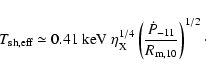
The magnetic equilibrium radius was estimated to be $80~\rm {km}$ due to the presence of iron line emission (Strohmayer & Imbrahim 2000) in which case for $\zeta\sim 0.004$ we get $\Delta P/P\sim 1.5\times 10^{-4}$ and $t_{\dot{P}}\sim 67$ days. However as discussed in Sect. 7.2.1 for an ionized atmosphere, redshift correction could move the radius to $30~\rm {\rm km}$ in which case a $\zeta\sim 0.1$ gives $\Delta P/P\sim 1.4\times 10^{-4}$ and $t_{\dot{P}}\sim 61$ days. This is in good agreement with what can be inferred from observations.

  
7.2.1 Iron line emission during bursts

Observations of Fe fluorescence lines in SGR 1900+14 (Strohmayer & Ibrahim 2000) are a key feature in our quark star model. As discussed in Ouyed et al. (2002) and Keränen et al. (2005), Fe and heavier metal production in the ejecta is significant during the formation of a quark star. Strohmayer & Ibrahim state that the distance from the star's surface, where the emission is created needs to be at least, $h\sim 80~\rm {km}$, to account for the lack of redshift. This distance gives an excellent confirmation to our model, as it corresponds to the distance of the shell which possess an Fe-rich atmosphere.

The atmosphere's column density can be calculated from Eq. (42) to be,

$$N_{\rm Fe} = 3.8\times 10^{24}\ {\rm cm}^{-2}\ R_{\rm m,10}... ...\left( \frac{kT_{\rm s, eff}}{1 ~{\rm keV}} \right)^{5/2}\cdot$$ (51)

This is sufficient to produce a strong $K_{\alpha}$ iron emission line (equivalent width >100 eV), when illuminated. Thus in our model, the Fe flourescent line is produced during bursts by the illumination of the shell's atmosphere.

  
7.3 X-ray to infrared flux ratio

Another observed feature in both SGRs and AXPs is the X-ray to infrared flux ratio correlations. The X-ray flux during the quiescent phase (induced by the magnetic field decay) and/or during the bursting phase (from accretion events) can be thermally reprocessed by the shell into the far infrared. However, the efficiency is too low due to the small shell size and cannot account for the observed values of $(\nu F_{\nu})_{\rm X}/(\nu F_{\nu})_{\rm IR}$ which are $\sim$150 for SGRs and $\sim$1500 for AXPs (e.g. Israel et al. 2003).

Alternatively one expects a much higher infrared flux related to vortex annihilation, which is always present in this model. The mechanism is synchrotron emission from mildly relativistic electrons accelerated by the magnetic reconnection events induced by vortex annihilation (see simulations in Ouyed et al. 2005). The X-rays are from the high energy electrons and the infrared from the low-energy electrons.

For a power-law electron energy distribution $N(E)\propto E^{-\gamma}$the optically thin synchrotron flux is given by $F_{\nu}\propto \nu^{-(\gamma -1)/2}$(Longair 1992). This implies

$$\frac{\left(\nu F_{\nu}\right)_{\rm X}}{(\nu F_{\nu})_{\rm IR... ...right)^{(3-\gamma)/2} \simeq (2\times 10^4)^{(3-\gamma)/2}\ .$$ (52)

For a typical index $\gamma=2$ this yields

$$\frac{(\nu F_{\nu})_{\rm X}}{(\nu F_{\nu})_{\rm IR}} \sim 140 .$$ (53)

In this model both $L_{\rm X}$ and $L_{\rm IR}$are proportional to $\dot{P}^2$ (see Eq. (30)) which also implies $L_{\rm IR}/L_{\rm X}$ is a constant. Synchrotron self-absorption at lower frequencies, low-energy electron losses, or a smaller index $\gamma$, all increase the $F_{\rm X}/F_{\rm IR}$ ratio, and may be the reason why AXPs show larger ratios than SGRs. During bursting episodes the vortex annihilation rate increases due to the spin-up induced by accretion increasing both $L_{\rm X}$and $L_{\rm IR}$, thus they remain correlated during bursts.

  
7.4 The hard spectrum/component in our model

Three of the four known SGRs have had hard spectrum (with photons in the MeV energy) giant flares. Before showing how this can be accounted for in our model, recall that in the case of quark stars the surface emissivity of photons with energies below $\hbar\omega_{\rm p}$ $\simeq$23 MeV ( $\omega_{\rm p}$: electromagnetic plasma frequency) is strongly suppressed (Alcock et al. 1986; Chmaj et al. 1991; Usov 1997). In Vogt et al. (2004) it was shown that average photon energies in quark stars in the CFL phase at temperatures T are $\sim$3T. Therefore, as soon as the surface temperature of the star cools below $T_{\rm a} = \hbar\omega_{\rm p}/3\simeq 7.7$ MeV, the photon emissivity is highly attenuated. This is studied in more details in Ouyed et al. (2005) where it was demonstrated that for temperatures above 7.7 MeV, neutrino cooling is dwarfed by the photons; i.e., photon emission/cooling dominates as long as the star cools from its initial temperature T₀>7.7 MeV to $T_{\rm a}=7.7$ MeV. For temperatures below 7.7 MeV, cooling is dictated by the slower neutrino processes.

To a first approximation, the increase in the star's temperature, $\Delta T_{\rm QS}$, following the accretion of shell pieces can be written as,

$$4\pi R_{\rm QS}^{2}\Delta R (1-\sin\theta_{\rm B}) c_{\rm v} \Delta T_{\rm QS} \simeq \eta \Delta m_{\rm sh} c^2 ,$$ (54)

where $c_{\rm v}= 7.8\times 10^{16} T_{\rm MeV}^3\ {\rm erg\ cm}^{-3}\ {\rm K}^{-1}$ is the star's specific heat as given in Ouyed et al. (2005). Also, $\Delta R$ is the thickness of the heated region in the polar caps. Since the pieces fall off above the neutral line (i.e. $\theta > \theta_{\rm B}$), the polar regions are the ones that are primarily heated in the process. The corresponding increase in temperature (assuming the initial star temperature is in the keV range) is then,

$$T_{\rm QS} \simeq 10~{\rm MeV} \frac{E_{\rm b, 45}^{3/16}}{\l... ... f^{1/4}(\alpha) R_{\rm QS, 10}^2 B_{15} \right)^{1/4}} \cdot$$ (55)

For $\theta_{\rm B}= 60^o$, $\alpha=1$, and $B_{15}\sim 1$, this implies that only accretion events with energy exceeding $E_{\rm b, c}\sim 2.8\times 10^{43}$ erg are capable of reheating the star above 7.7 MeV, allowing MeV photons to be generated and escape the star. Thus our model naturally explains why only the rare giant bursts emit a hard-spectrum.

The escaping photons are thermalized and cool the star at a rate given by $4\pi (1-\sin\theta_{\rm B}) R_{\rm QS}^2 \Delta R c_{\rm v} \partial T_{\rm QS}/\partial t = - 4\pi R_{\rm QS}^2 \sigma T_{\rm QS}^4$ which leads to a cooling time of,

$$t_{\rm c, QS} \sim 0.03\ {\rm ms}~ \frac{(1-\sin\theta_{\rm... ...{E_{\rm b,45}^{1/4}} \log{\frac{T_{\rm QS}}{T_{\rm a}}}\cdot$$ (56)

As the high energy photons escape into the magnetosphere they interact with lower energy photons and $\rm (e^+e^-)$ pairs, and so become thermalized to about $\sim$1 MeV. The $\rm (e^+e^-)$ pairs could be due to the radiation from the magnetic field decay which occurs outside the surface of the quark star. We note that the radiation produced by accretion is from the conversion of baryons to quarks at the surface which also releases photons at the surface (half of this radiation heats the quark matter inside the star while the other half is radiated promptly). We have not studied these emission mechanisms in details but we are currently investigating mechanisms for thermalizing the escaping radiation, and the nature of the resulting spectrum. We can simply argue for now that the radiation mechanisms should be similar to those for a pair-dominated fireball in an optically thick environment.

  
7.5 Summary of outstanding SGR/AXP questions

We summarize this section by attempting to test our model against the open issues related to SGRs/AXPs as discussed in the literature (i.e. Israel 2006). These open issues are enumerated below.

1.

Are the SGRs/AXPs engines born with milliseconds periods?

Allen & Hovarth (2004) and Vink & Kuiper (2006) give good evidence in two cases for normal energy supernova shells around an AXP (1E1841-045) and an SGR (0526-66), which implies birth periods larger than tens of milliseconds. In our model there is no need for rapid rotation at birth.

2.

What differentiates the two types (giant and regular) of bursts? How does the boxing day, SGR 1806-20 event fit in this picture?

A giant burst is due to the shell losing a larger fraction of its mass as it moves towards the star, parameterized in our model by $\alpha\sim 1$. Regular bursts, $\alpha \ll 1$, are due to smaller pieces breaking off the neutral line as the shell oscillates around its equilibrium position. For SGR 1806-20 we argue the boxing day event is one of the first events experienced by this object following its birth. Moreover, our model predicts (via Eq. (21)) that we should continue to see a decreasing trend in both the burst intensity and frequency going from younger to older objects.

3.

Why are the IR and X-ray variability correlated during flares? Is the far-IR emission due to a passive disk? Why passive? Why disk?

The far-IR emission and the correlation with the X-ray emission can simply be explained as synchrotron emission from the high-energy and low-energy electrons (see Sect. 7.3). Our disk is in fact an iron-rich shell. It is passive because it is degenerate and for most of its lifetime it remains in equilibrium at $R_{\rm m}$, co-rotating with the star.

4.

Is there any connection between AXPs/SGRs and high-B radio pulsars?

AXPs/SGRs are quark stars and high-B radio pulsars are neutron stars that have not gone through a QN phase, probably because their core densities never reached deconfinement values (see Staff et al. 2006).

5.

What is the origin of the hard X-ray spectrum in AXPs/SGRs?

The hard X-ray spectrum in our model can be explained as MeV photons generated in the outer layers of the star. These photon bursts can only occur for accretion events capable of heating the star above 7.7 MeV. We find that only bursts with energies above 10⁴³ erg can do so (see Sect. 7.4), thus explaining why only the giant SGR flares show a hard spectrum.

6.

Why do the spin-down ages and the supernova ages differ?

In our model the difference can be explained by the time it takes the neutron star to reach deconfinement/nucleation densities as discussed in Sect. 4.4. Simply put, the supernova age is the time for the neutron star to reach quark deconfinment densities and experience a quark-nova, plus the time needed for strange quark nucleation ( $t_{\rm SN} = t_{\rm QN} + t_{\rm nucl.}$).

7.

What are the progenitors of AXPs/SGRs and why are they located in dense ISM?

Massive stars (near the black hole line) exploding in high density ISM are most likely to lead to massive compact remnants. The high density ISM will confine the massive progenitor winds much closer to the star, causing the deceleration of the blast wave, and initiating the reverse shock inside the remnant (Truelove & McKee 1999). This would lead to more massive compact stars which are more likely to turn directly into quark stars.

  
8 XDINs in our model

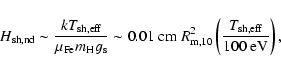
In our model X-ray Dim Isolated Neutron Stars (XDINs) are old SGRs/AXPs that have gone through their most active bursting phase and are left with a thin shell in stable equilibrium at $R_{\rm m}$. We start by summarizing the observed and measured features of XDINs before we apply our model to these intriguing objects.

8.1 Properties of XDINs

These dim ( $L_{\rm X}\sim 10^{31}\ {\rm erg\ s}^{-1}$) isolated neutron stars are nearby at around 100-300 pc and show no SNR association. Three of them have known proper motions that are too fast to accrete. The main common properties of the "magnificent seven'' can be summarized as follows (see Haberl 2005 and references therein): (i) the blackbody: the X-ray spectra of XDINs obtained by the ROSAT PSPC are all consistent with blackbody emission. The soft X-ray spectra have a temperature in the range of 40-110 eV. They show no non-thermal component; (ii) the Absorption lines: the XMM-Newton spectra can be best modeled with a Planckian continuum including a broad, Gaussian shaped absorption line. The line centroid energies are in the range 100-700 eV. The depth of the absorption line (or the equivalent width) was found to vary with pulse phase. It has been suggested in the literature that these absorption lines can be best explained as proton cyclotron resonance absorption features in the 0.1-1 keV band with field strength in the range of $2\times 10^{13}$- $2\times 10^{14}$ G (Zane et al. 2001; Zavlin & Pavlov 2002) with the line broadening explained as due to the variation of the magnetic field over the neutron star surface; (iii) the optical excess: they show optical excess compared to the X-ray blackbody. In other words at optical wavelengths they show a factor of about 3-14 excess when compared to the extrapolation from X-rays (Pons et al. 2002; Motch & Haberl 1998; Haberl et al. 2004; van Kerkwijk et al. 2004); (iv) the Lack of radio-emission: it has been argued that the lack of pulsed radio-emission is because their radio beam is very narrow due to the large light cylinder radius (i.e., large periods). However, there exist radio-pulsars with similar magnetic field strengths and periods (e.g. Camilo et al. 2000) that are active in the radio. In our model, the lack of radio pulsation is due to the fact that quark stars in the CFL phase, unlike neutron stars, become aligned-rotators following the QN (see Ouyed et al. 2005). We now go on to discuss the remaining properties.

Table 2: Observed features of the X-ray dim radio-quiet isolated neutron stars $^{\ddag\ddag }$.

8.2 The two-component blackbody

As discussed in Sect. 5.1, the first blackbody temperature is set by the X-ray continuum luminosity from the surface of the quark star,

$$T_{\rm BB} \simeq 41.0 \ {\rm eV}\ \left(\frac{\dot{P}_{-13}}{R_{\rm QS, 10}}\right)^{1/2}\cdot$$ (57)

Note that the spin-down is in units of 10^-13 s/s reflective of what has been measured for XDINs. The observer would see an emitting region with a corresponding blackbody radius $R_{\rm BB} = R_{\rm QS} \sqrt{1-\sin\theta_{\rm B}}\sim 4.4$ km using our fiducial value $\theta_{\rm B}=60\hbox{$^\circ$ }$. Interestingly, these are the same values as inferred for RX J1856 (e.g. Burwitz et al. 2003) and RXJ0720 (e.g. Haberl 2004).

Similarly, the effective shell temperature (the second blackbody) is

$$T_{\rm sh,eff} \simeq 41.0 \ {\rm eV}\ \left(\frac{\dot{P}_{... ...\left( \frac{R_{\rm QS, 10}}{R_{\rm m, 10}} \right)^{1/2}\cdot$$ (58)

8.3 Absorption lines

Since $R_{\rm m} > R_{\rm QS}$ in our model it implies $T_{\rm sh, eff} < T_{\rm BB}$which means that the shell will act as an absorber of the hotter X-ray blackbody. The maximum density, $\rho_{\rm s,nd}$, of the shell below which the gas is non-degenerate is found by setting $T_{\rm sh,eff}= T_{\rm Fermi}$, or, $\rho_{\rm sh,nd} \simeq 54\ {\rm g\ cm}^{-3}\times \left(T_{\rm sh,eff}/100\; {\rm eV}\right)^{3/2}$. The scale height of the non-degenerate, upper layers, of the shell can be estimated to be

$$H_{\rm sh,nd} \sim\frac{ k T_{\rm sh,eff}}{\mu_{\rm Fe} m_{\r... ... 10}^2 \left( \frac{T_{\rm sh, eff}}{100\; {\rm eV}}\right) ,$$ (59)

implying a mass of the non-degenerate portion of the shell of

$$m_{\rm sh,nd} 4\pi R_{\rm m}^2 \sin\theta_{\rm B} \ H_{\rm sh, nd} \rho_{\rm s, nd}$$ = (60)

$$\sim 3.1\times 10^{12} \ {\rm g} \ R_{\rm m,10}^4 \left( \frac{T_{\rm sh, eff}}{100\; {\rm eV}}\right)^{5/2} ,$$

with an optically thick column density,

 

$$N_{\rm Fe} \simeq \frac{H_{\rm s,nd}\rho_{\rm s,nd}}{(56 m_{\rm H})} \sim 2.1\times... ...-2}\ R_{\rm m,10}^2 \left( \frac{T_{\rm sh, eff}}{100\; {\rm eV}} \right)^{5/2}$$ (61)

$$\sim 2.1\times 10^{18}\ {\rm cm}^{-2}\ R_{\rm m,10}^{3/4} \left( \frac{T_{\rm BB}}{100\; {\rm eV}} \right)^{5/2} \cdot$$

Iron photospheric models have been calculated by Rajagopal et al. (1997) for magnetic field strengths as derived for XDINSs in our model (i.e. $B=\sqrt{3\kappa P\dot{P}}\sim 10^{13}$ G). Despite the fact that these calculations are only done in Hartree-Fock approximation the results show absorption features in the blackbody spectra, at energies 300 eV and above, reminiscent of the lines in XDINSs (see Fig. 3 in Rajagopal et al. 1997; see also discussion in Neuhauser et al. 1987). Careful attention to Fig. 3 in Rajagopal et al. (1997) shows that the lines start to disappear at temperature between 30 eV and 80 eV. Interestingly, this temperature effect may explain the absence of absorption line in the two XDINSs showing the lowest blackbody temperature namely, RX J0420.0-5022 with $kT_{\rm bb}\sim 40$ eV and RX J1856.5-3754 (the brightest or closest of the XDINs) with $kT_{\rm bb}\sim 60$ eV. We thus suggest that the iron shell in our model provids the conditions necessary to explain the absorption lines as iron lines. In this respect, the iron atmosphere explanation of the spectrum suggests that younger (i.e. hotter) objects of the same type should be observed with a richer line spectrum.

8.4 The optical excess

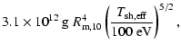The shell's solid angle, $4\pi\sin\theta_{\rm B}$, is essentially providing the excess optical emission. In the simplest case, one assumes a scattering atmosphere isotropizes the optical emitted flux from the QS (i.e. blackbody tail) and the shell. Then the ratio between the total optical flux and the optical contribution from the tail of the blackbody can be expressed as

$$\frac{F_{\rm opt, tot}}{F_{\rm opt, tail}} 1 + \frac{F_{\rm opt,sh}}{F_{\rm opt, tail}}$$ = (62)

$$1 + \frac{4\pi \sin\theta_{\rm B}}{4\pi (1-\sin\theta_{\rm B})} =\frac{1}{1-\sin\theta_{\rm B}}\sim 7 .$$ =

In other words, the optical excess is a direct measure of the angle subtended by the shell. This also means a one-to-one correspondence between the optical excess and the size of the emitting spot in our model expressed as

$$\frac{F_{\rm opt, tot}}{F_{\rm opt, tail}} = \frac{1}{1-\sin\theta_{\rm B}} = \left(\frac{R_{\rm QS}}{R_{\rm BB}}\right)^2 .$$ (63)

For example for RXJ1856 $R_{\rm BB}\sim 4.4$ km has been derived from observations. Assuming a quark star radius of about 10 km, our model would then predict an optical excess of $(10/4.4)^2\sim 5$ which is very close to the factor 5-7 measured from the current optical data and the LETG spectrum (Haberl 2004). The radius of the emitting area in the case of RXJ0720.4 has also been estimated to be 4.4-4.8 km (for a distance of 300 pc) which should give an optical excess of $\sim$5 in our model and similar to what is observed (see Table 2).

  
9 Conclusion

In this paper we present a new model for SGRs and AXPs with possible applications to XDINs. This novel idea relies on the formation of bare CFL quark stars (within the quark-nova scenario) as the underlying engine, with the parent neutron star's crust material surrounding it. Despite the simplifications we have employed to study the dynamics of this ejected shell, specifically how it reaches the equilibrium radius and how it evolves once it is there, our model has a number of attractive features that can account for many observed SGR, AXP, and perhaps XDIN properties.

Missing from our study is the proper treatment of three-dimensional instabilities acting on the shell, such as Raleigh-Taylor or oscillations. Due to the high conductivity of the shell we expect the Raliegh-Taylor to not operate on very fast timescales, and any radial oscillations to be severly damped as the conducting shell will maintain the magnetic flux enclosed within. However, azimuthal oscillations may have a significant effect. For a more accuarate description, the dynamics of the shell will require numerical simulations, and is left as future work.

Acknowledgements

We thank K. Mori and P. Jaikumar for insightful discussions. This research is supported by grants from the Natural Science and Engineering Research Council of Canada (NSERC).

References

• Alcock, C., Farhi, E., & Olinto, A. 1986, ApJ, 310, 261 [NASA ADS] [CrossRef] (In the text)
• Allen, M. P., & Hovarth, J. E. 2004, ApJ, 616, 346 [NASA ADS] [CrossRef] (In the text)
• Bombaci, I., Parenti, I., & Vidaña, I. 2004, ApJ, 614, 314 [NASA ADS] [CrossRef] (In the text)
• Burwitz, V., Haberl, F., Neuhäuser, R., et al. 2003, A&A, 399, 1109 [NASA ADS] [CrossRef] [EDP Sciences] (In the text)
• Camilo, F., Thorsett, S. E., & Kulkarni, S. R. 1994, ApJ, 421, L15 [NASA ADS] [CrossRef]
• Camilo, F., Kaspi, V. M., Lyne, A. G., et al. 2003, A&A, 541, 367
• Chmaj, T., Haensel, P., & Slominski, W. 1991, Nucl. Phys. B Proc. Suppl., 24, 40 [NASA ADS] [CrossRef] (In the text)
• Datta, B., Thampan, A. V., & Bhattacharya, D. 1995, J. Astrophys. Astron., 16, 375 [NASA ADS] (In the text)
• Frank, J., King, A., & Raine, D. 1992, Accretion Power in Astrophysics (Cambridge: Cambridge Univ. Press)
• Ferrer, E. J., de la Incera, V., & Manuel, C. 2005, Phys. Rev. Lett., 95, 152002 [NASA ADS] [CrossRef] (In the text)
• Gavriil, F. P., Kaspi, V. M., & Woods, P. M. 2002, Nature, 419, 142 [NASA ADS] [CrossRef]
• Glendenning, N. K. 1997, Compact stars (Springer)
• Haberl, F. 2002, Mem. S. A. It., 1, 1
• Haberl, F. 2004, Adv. Space Res., 33, 638 [NASA ADS] (In the text)
• Haberl, F. 2005, MPE Rep., 288, 39 [arXiv:astro-ph/0510480] (In the text)
• Haberl, F., Zavlin, V. E., Trümper, J., & Burwitz, V. 2004, A&A, 419, 1077 [NASA ADS] [CrossRef] [EDP Sciences]
• Hulleman, F., van Kerkwijk, M. H., & Kulkarni, S. R. 2004, A&A, 416, 1037 [NASA ADS] [CrossRef] [EDP Sciences]
• Illarionov, A. F., & Sunyaev, R. A. 1975, A&A, 39, 185 [NASA ADS] (In the text)
• Israel, G. L., et al. 2003, ApJ, 589, L93 [NASA ADS] [CrossRef] (In the text)
• Iwazaki, A. 2005, Phys. Rev. D, 72, 114003 [NASA ADS] [CrossRef] (In the text)
• Jaikumar, P., Otsuki, K., Meyer, B. S., & Ouyed, R. 2006, submitted [arXiv:nucl-th/0610013] (In the text)
• Kaspi, V. M., Lackey, J. R., & Chakrabarty, D. 2000, ApJ, 537, L31 [NASA ADS] [CrossRef]
• Keränen, P., & Ouyed, R. 2003, A&A, 407, L51 [NASA ADS] [CrossRef] [EDP Sciences] (In the text)
• Keränen, P., Ouyed, R., & Jaikumar, P. 2005, ApJ, 618, 485 [NASA ADS] [CrossRef] (In the text)
• Lang, K. R. 1974 (New York: Springer-Verlag New York, Inc.), 760 (In the text)
• Lugones, G., & Horvath, J. E. 2002, Phys. Rev. D, 66, 074017 [NASA ADS] [CrossRef] (In the text)
• Longair, M. S. 1992, High Energy Astrophysics, ed. by Malcolm S. Longair, 436 Cambridge (UK: Cambridge University Press) (In the text)
• Mazets, E. P., Golenetskii, S. V., Ilinskii, V. N., Aptekar, R. L., & Guryan, I. A. 1979, Nature, 282, 587 [NASA ADS] [CrossRef] (In the text)
• Motch, C., & Haberl, F. 1998, A&A, 333, L59 [NASA ADS] (In the text)
• Neuhauser, D., et al. 1987, Phys. Rev. A, 36, 4163 [NASA ADS] [CrossRef] (In the text)
• Niebergal, B., Ouyed, R., & Leahy, D. 2006, ApJ, 646, L17 [NASA ADS] [CrossRef] (In the text)
• Ouyed, R., Dey, J., & Dey, M. 2002, A&A, 390, L39 [NASA ADS] [CrossRef] [EDP Sciences] (In the text)
• Ouyed, R., Elgarøy, Ø., Dahle, H., & Keränen, P. 2004, A&A, 420, 1025 [NASA ADS] [CrossRef] [EDP Sciences] (In the text)
• Ouyed, R., Niebergal, B., Dobler, W., & Leahy, D. 2005, ApJ, in Press [arXiv:astro-ph/0510691] (In the text)
• Ouyed, R., Rapp, R., & Vogt, C. 2005, ApJ, 632, 1001 [NASA ADS] [CrossRef]
• Ouyed, R., Leahy, D., & Niebergal, B. 2006 [arXiv:astro-ph/0611133] (In the text)
• Palmer, D. M. 2002, Mem. Soc. Astron. It., 73, 578 [NASA ADS] (In the text)
• Palmer, D. M., Barthelmy, J., Gehrals, N., et al. 2005, Nature, 434, 1107 [NASA ADS] [CrossRef] (In the text)
• Pathria, R. K. 1996, Statistical Mechanics, 2nd edn (Butterworth-Heinemann Publishing Group.)
• Pons, J. A., Walter, F. M., Lattimer, J. M., et al. 2002, ApJ, 564, 981 [NASA ADS] [CrossRef] (In the text)
• Rajagopal, M., Romani, R. W., & Miller, C. M. 1997, ApJ, 479, 347 [NASA ADS] [CrossRef] (In the text)
• Rajagopal, K., & Wilczek, F. 2001, Phys. Rev. Lett., 86, 3492 [NASA ADS] [CrossRef] (In the text)
• Schwartzman, V. F. 1970, Radiofizika, 13, 1852 (In the text)
• Staff, J. E., Ouyed, R., & Jaikumar, P. 2006, ApJ, 645, L145 [NASA ADS] [CrossRef] (In the text)
• Truelove, J. K., & McKee, C. F. 1999, ApJS, 120, 299 [NASA ADS] [CrossRef] (In the text)
• Trümper, J. E. 2005 [arXiv:astro-ph/0502457]
• Usov, V. V. 1997, ApJ, 481, L107 [NASA ADS] [CrossRef] (In the text)
• Usov, V. V. 2004, Phys. Rev. D, 70, 067301 [NASA ADS] [CrossRef] (In the text)
• van Kerkwijk, M. H., Kaplan, D. L., Durant, M., Kulkarni, S., & Paerels, F. 2004, ApJ, 608, 432 [NASA ADS] [CrossRef] (In the text)
• Vink, J., & Kuiper, L. 2006, MNRAS, 370, L41 [NASA ADS] (In the text)
• Woods, P. M., Kouveliotou, C., van Paradijs, J., et al. 1999, ApJ, 524, L55 [NASA ADS] [CrossRef] (In the text)
• Zane, S., Turolla, R., Stella, L., & Treves, A. 2001, ApJ, 560, 384 [NASA ADS] [CrossRef] (In the text)
• Zavlin, V. E., & Pavlov, G. G. 2002, in Neutron Stars, Pulsars, and Supernova Remnants, ed. W. Becker, H. Lesch, & J. Trümper, MPE Rep., 278, 263 (In the text)

 

  
Online Material

Table 1: Observed features of SGRs and AXPs (Only AXPs and SGRs with measured P and $\dot{P}$ are listed)⁺.