![[*]](/icons/foot_motif.gif)
A&A 456, 117-129 (2006)
DOI: 10.1051/0004-6361:20054649
I. Agudo1 - T. P. Krichbaum1 - H. Ungerechts2 - A. Kraus1 - A. Witzel1 - E. Angelakis1 - L. Fuhrmann1,3,4 - U. Bach1,4 - S. Britzen1 - J. A. Zensus1 - S. J. Wagner5 - L. Ostorero5,6 - E. Ferrero5 - J. Gracia7 - M. Grewing8
1 - Max-Planck-Institut für Radioastronomie,
Auf dem Hügel 69,
53121 Bonn, Germany
2 -
Instituto de Radio Astronomía Milimétrica,
Avenida Divina Pastora 7, Local 20,
18012 Granada, Spain
3 -
Dipartimento di Fisica, Università di Perugia,
via A. Pascoli, 06123 Perugia, Italy
4 -
INAF, Osservatorio Astronomico di Torino,
via Osservatorio 20, 10025 Pino Torinese (TO), Italy
5 -
Landessternwarte Heidelberg-Königstuhl, Königstuhl,
69117 Heidelberg, Germany
6 -
Tuorla Observatory, University of Turku, Väisäläntie
20, 21500 Piikkiö, Finland
7 -
Department of Physics, University of Athens,
Panepistimiopolis, 157 84 Zografos,
Athens, Greece
8 -
Institut de Radio Astronomie Millimétrique,
300 rue de la Piscine, Domaine Universitaire
de Grenoble, 38406 Saint Martin d'Hères, France
Received 5 December 2005 / Accepted 31 May 2006
Abstract
We report on a densely time sampled polarimetric flux density
monitoring of the BL Lac object S5 0716+71 at 86 GHz and 229 GHz.
The source was observed with the IRAM 30 m telescope at Pico
Veleta within a coordinated multi-frequency observing campaign,
which was centred around a 500 ks INTEGRAL observation during November 10 to 16, 2003. The aim of this campaign was to search
for signatures of inverse-Compton catastrophes through the
observation of the broad-band variability of the source.
At 86 GHz, S5 0716+71 showed no intra-day variability,
but showed remarkable inter-day variability with a flux density
increase of 34% during the first four observing days,
which cannot be explained by source extrinsic causes.
At this frequency,
making use of a new calibration strategy, we reach a relative
rms accuracy of the flux density measurements of 1.2%.
Although the flux density variability at 229 GHz was consistent
with that at 86 GHz, the larger measurement errors at
229 GHz do not allow us to detect, with high confidence,
inter-day variations at this frequency. At 86 GHz, the
linear polarization fraction of S5 0716+71 was unusually large
 .
Inter-day variability in linear polarization at 86 GHz,
with significance level
.
Inter-day variability in linear polarization at 86 GHz,
with significance level
 ;
;
 % and
% and
 ,
was observed
during the first four observing days.
From the total flux density variations at the synchrotron turnover
frequency (
,
was observed
during the first four observing days.
From the total flux density variations at the synchrotron turnover
frequency (
 )
we compute an apparent brightness
temperature
)
we compute an apparent brightness
temperature
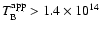 K
at a redshift of 0.3, which exceeds by two orders of magnitude
the inverse-Compton limit.
A relativistic correction for
K
at a redshift of 0.3, which exceeds by two orders of magnitude
the inverse-Compton limit.
A relativistic correction for
 with a
Doppler factor
with a
Doppler factor
 brings the observed brightness
temperature down to the inverse Compton limit.
A more accurate lower limit of
brings the observed brightness
temperature down to the inverse Compton limit.
A more accurate lower limit of
 ,
consistent with
previous estimates from VLBI observations, is obtained
from the comparison of the 86 GHz synchrotron flux density
and the upper limits for the synchrotron self-Compton
flux density obtained from the INTEGRAL observations.
The relativistic beaming of the emission by this high Doppler
factor explains the non-detection of "catastrophic''
inverse-Compton avalanches by INTEGRAL.
,
consistent with
previous estimates from VLBI observations, is obtained
from the comparison of the 86 GHz synchrotron flux density
and the upper limits for the synchrotron self-Compton
flux density obtained from the INTEGRAL observations.
The relativistic beaming of the emission by this high Doppler
factor explains the non-detection of "catastrophic''
inverse-Compton avalanches by INTEGRAL.
Key words: galaxies: active - galaxies: BL Lacertae objects: general - galaxies: BL Lacertae objects: individual: S5 0716+71 - radio continuum: galaxies - radiation mechanisms: non-thermal - polarization
The effect of intra-day variability (IDV) of radio loud active
galactic nuclei (AGN) in the radio bands was discovered in 1986
(Witzel et al. 1986; Heeschen et al. 1987) and
since then led to controversial discussions about its physical
origin.
Most of the objects presenting radio IDV appear
compact -when are observed in the radio and optical bands -,
their relativistic jets are highly core-dominated on VLBI
scales and exhibit high brightness temperatures (e.g.
Wagner & Witzel 1995).
IDV is a common phenomenon in extragalactic flat
spectrum radio sources and is observed, at centimetre wavelengths,
in about 10% to 25% of all objects of this class
(Quirrenbach et al. 1992;
Kedziora-Chudczer et al. 2001; Lovell et al. 2003).
The "classical IDV'' (of type II, as defined in Heeschen et al.
1987) is characterised by variability amplitudes
 % and variability time-scales between 0.5 days
and 2 days.
In parallel to the variability of the total flux density,
similar or even faster variations of the linear polarization
(Quirrenbach et al. 1989; Kraus et al.
1999a,b, 2003) and of the
circular polarization (Macquart et al. 2000)
are observed.
Intensity and polarization variations can be correlated or
anti-correlated (e.g. Wagner et al. 1996;
Macquart et al. 2000; Qian et al. 2002).
% and variability time-scales between 0.5 days
and 2 days.
In parallel to the variability of the total flux density,
similar or even faster variations of the linear polarization
(Quirrenbach et al. 1989; Kraus et al.
1999a,b, 2003) and of the
circular polarization (Macquart et al. 2000)
are observed.
Intensity and polarization variations can be correlated or
anti-correlated (e.g. Wagner et al. 1996;
Macquart et al. 2000; Qian et al. 2002).
Observations of IDV sources in the radio and millimetre
bands are particularly important, since they reveal the
highest apparent brightness temperatures
(
 ;
e.g. Readhead 1994).
However, the observed radio emission might also be severely
affected by interstellar scintillation (ISS), which is unavoidable
because of the small intrinsic sizes of IDV sources (Rickett
1990).
It is known that, for high Galactic latitude blazars,
the amplitude of IDV due to the
effect of interstellar scintillation rapidly decreases
with frequency for
;
e.g. Readhead 1994).
However, the observed radio emission might also be severely
affected by interstellar scintillation (ISS), which is unavoidable
because of the small intrinsic sizes of IDV sources (Rickett
1990).
It is known that, for high Galactic latitude blazars,
the amplitude of IDV due to the
effect of interstellar scintillation rapidly decreases
with frequency for  GHz (e.g. Rickett 1990;
Rickett et al. 1995; Beckert et al. 2002).
In such case and for a source whose size is constant with
frequency, the ISS-induced variability amplitude scales as
GHz (e.g. Rickett 1990;
Rickett et al. 1995; Beckert et al. 2002).
In such case and for a source whose size is constant with
frequency, the ISS-induced variability amplitude scales as
 (e.g. Beckert et al. 2002).
Hence, any rapid and large amplitude source
variability seen at millimetre (or shorter) wavelengths should
not be strongly affected by ISS.
Therefore, monitoring of IDV sources at mm-bands is particularly
important to determine whether the observed IDV is
mainly source extrinsic (scintillation), due to source
intrinsic processes, or a mixture of both.
(e.g. Beckert et al. 2002).
Hence, any rapid and large amplitude source
variability seen at millimetre (or shorter) wavelengths should
not be strongly affected by ISS.
Therefore, monitoring of IDV sources at mm-bands is particularly
important to determine whether the observed IDV is
mainly source extrinsic (scintillation), due to source
intrinsic processes, or a mixture of both.
S5 0716+71 (hereafter 0716+714) is an extremely active BL Lac object which varies on time scales from less than one hour to months, from radio to X-rays (e.g. Wagner et al. 1996; Kraus et al. 2003; Raiteri et al. 2003). Although the optical spectrum of 0716+714 appears featureless, even with 4 m class telescopes, the absence of any signature of a host galaxy (in deep images) sets a lower limit to its redshift of z>0.3 (Wagner et al. 1996). Therefore, only lower limits to the brightness temperature of the source can be derived. The strongest constraint on the brightness temperature of this source comes from the observed short variability time-scales at radio wavelengths, which sets, via the causality argument, an upper limit to the source size of a few tens of micro-arcseconds. During the last decade the source has been observed repeatedly in simultaneous centimetre wavelength campaigns (Wagner et al. 1990, 1996; Otterbein et al. 1999; Kraus et al. 2003; Raiteri et al. 2003), during which it typically showed IDV. 0716+714 is the only IDV source which has shown simultaneous variability-time-scale transitions in the radio and optical bands, which have been interpreted as evidence for source intrinsic variability (Quirrenbach et al. 1991; Wagner & Witzel 1995; Qian et al. 1996). The correlation between the radio spectral index and the optical flux suggested that the radiation was produced by the same particle population (Qian et al. 1996). Additional arguments for the relevance of the intrinsic origin of the IDV in 0716+714 come from the variability amplitude, which increases from radio to optical, and the recently detected IDV at a wavelength of 9 mm (Kraus et al. 2003). Both effects contradict expectation for the frequency dependence of ISS.
If IDV is produced by the intrinsic properties of AGN,
very small angular sizes of the emitting regions
(of a few micro-arcseconds) are inferred from their short
variability time-scales.
This usually implies apparent brightness temperatures several
orders of magnitude larger than the inverse-Compton (IC)
limit (
 K, Kellermann & Pauliny-Toth 1969;
Readhead 1994; Kellermann 2003).
For incoherent synchrotron
sources of radiation, this limit could be violated only during
short time ranges, because the high energy photon densities
at the
IC-limit should lead to the rapid cooling of the
emitting region through the IC scattering of the synchrotron
radiation. This process is known as the inverse-Compton
catastrophe.
The relativistic beaming of the radiation coming from the
emitting region (Rees 1966) has been proposed as a
likely cause to explain the systematic violation of the
IC-limit (e.g. Wagner & Witzel 1995).
Other scenarios, as coherent synchrotron radiation, which
is an unconventional but not impossible process in AGN, have
been proposed (e.g. Benford 1992).
However, the inverse-Compton catastrophe scenario cannot
still be ruled out (Wagner & Witzel 1995).
K, Kellermann & Pauliny-Toth 1969;
Readhead 1994; Kellermann 2003).
For incoherent synchrotron
sources of radiation, this limit could be violated only during
short time ranges, because the high energy photon densities
at the
IC-limit should lead to the rapid cooling of the
emitting region through the IC scattering of the synchrotron
radiation. This process is known as the inverse-Compton
catastrophe.
The relativistic beaming of the radiation coming from the
emitting region (Rees 1966) has been proposed as a
likely cause to explain the systematic violation of the
IC-limit (e.g. Wagner & Witzel 1995).
Other scenarios, as coherent synchrotron radiation, which
is an unconventional but not impossible process in AGN, have
been proposed (e.g. Benford 1992).
However, the inverse-Compton catastrophe scenario cannot
still be ruled out (Wagner & Witzel 1995).
A coordinated broad-band observing campaign
- centred around a 500 ks INTEGRAL observation
during November 10 to 16, 2003 - was performed to search
for signatures of inverse-Compton catastrophes on a flaring
state of 0716+714 through the correlation of the broad-band
variability of the source.
The ground-based observations were performed
with the VLBA, the Effelsberg 100 m, the Metsähovi 13.7 m,
the IRAM 30 m, the JCMT, the HHT, and the Kitt Peak 12 m
telescopes and the optical-IR telescopes of the
WEBT collaboration.
The first analysis of the broad-band (from radio to soft
 -rays) observations (Ostorero et al. 2006)
do not show obvious correlation between the intra-day optical
variability and the inter-day radio variability displayed by
the source. Although the apparent brightness temperatures of
0716+714 largely exceeded the IC-limit
at radio wavelengths, no evidence of IC avalanches
was seen in the INTEGRAL data.
-rays) observations (Ostorero et al. 2006)
do not show obvious correlation between the intra-day optical
variability and the inter-day radio variability displayed by
the source. Although the apparent brightness temperatures of
0716+714 largely exceeded the IC-limit
at radio wavelengths, no evidence of IC avalanches
was seen in the INTEGRAL data.
In this paper we report on the results and implications of the first polarimetric millimetre wavelength IDV observations of 0716+714, which were performed (within the above-mentioned campaign) with the IRAM 30 m radio telescope during the period November 10 to 18, 2003. A combined discussion of the radio, millimetre and sub-millimetre single dish data set will be presented by Fuhrmann et al. (in prep.). Forthcoming papers will describe more detailed analysis of the optical observations and more sophisticated theoretical modelling of the broad-band data set.
The observations presented here were specially planned to achieve
accurate measurements of the total flux density
with a typical temporal resolution better than 1 h.
To achieve this goal, we observed 0716+714 and a number of suitable
calibrators continuously for  18 h on each day during November
10 to 18, 2003, using the IRAM 30 m telescope at Pico Veleta (Granada,
Spain).
The observations were interrupted by intervals where the elevation of
the program source was lower than
18 h on each day during November
10 to 18, 2003, using the IRAM 30 m telescope at Pico Veleta (Granada,
Spain).
The observations were interrupted by intervals where the elevation of
the program source was lower than
 or when the weather
conditions were inappropriate for 86 GHz observations. Under these
conditions, accurate antenna and gain calibrations were not possible.
or when the weather
conditions were inappropriate for 86 GHz observations. Under these
conditions, accurate antenna and gain calibrations were not possible.
The receiver-cabin optic system of the IRAM 30 m telescope is
optimised to observe with up to four different receivers at the same time
(Wild 1999).
We made use of the A100, A230, B100 and B230 heterodyne receivers
of the telescope, which simultaneously observed at both
86 GHz (A100 and B100, at
 mm, where
  is
the wavelength) and 229 GHz (A230 and B230, at
is
the wavelength) and 229 GHz (A230 and B230, at
 mm).
This standard observing set-up uses a grid to divide the incoming
signal into two orthogonal linear polarizations and then two
Martin-Pupplet interferometers (one per polarization) to split the
86 GHz and the 229 GHz frequency bands.
Hence, at each observing band, the A- and B-receivers were sensitive
to two orthogonal linear polarizations.
This allowed us to obtain linear polarization information at 86 GHz.
Receiver A230 was not stable enough to provide reliable measurements
and hence we lost the polarization information at 229 GHz.
The observing bandwidths at 86 GHz and 229 GHz were 0.5 GHz and
1 GHz, and the typical single side band system temperatures
were 100 K and 400 K, respectively.
mm).
This standard observing set-up uses a grid to divide the incoming
signal into two orthogonal linear polarizations and then two
Martin-Pupplet interferometers (one per polarization) to split the
86 GHz and the 229 GHz frequency bands.
Hence, at each observing band, the A- and B-receivers were sensitive
to two orthogonal linear polarizations.
This allowed us to obtain linear polarization information at 86 GHz.
Receiver A230 was not stable enough to provide reliable measurements
and hence we lost the polarization information at 229 GHz.
The observing bandwidths at 86 GHz and 229 GHz were 0.5 GHz and
1 GHz, and the typical single side band system temperatures
were 100 K and 400 K, respectively.
All the measurements were performed in "beam-switching'' mode,
using a chopper wheel to subtract the emission contribution from
the sky.
During the continuous chopping (at a frequency of  7 Hz)
the telescope beam was moved to a 70
7 Hz)
the telescope beam was moved to a 70
 off-position.
The individual measurements were performed by
repeated cross-scans
over the source position in azimuth and elevation.
The number of sub-scans in each measurement and for each source was
chosen according to the flux density of the source, with more
sub-scans on the fainter objects.
For technical reasons, the number of sub-scans were multiples of
four and ranged between 4 and 16.
0716+714 was observed with a "duty cycle" of about
1 to 2 measurements every 60 min.
Also six bright and point-like extragalactic
radio sources (S5 0212+735, S5 0633+734,
S5 0836+710, S4 1642+690, S5 1803+784, S5 1928+738, which will be called hereafter by their
catalogue codes) were observed with a duty cycle
of at least one measurement every hour.
Their known variability characteristics at
cm-wavelengths and location on the sky allowed us to assume
that they were non-variable on time-scales of days and
so they were suitable as secondary calibrators.
For the determination of the absolute flux density scale,
we observed two planets (Mars and Uranus)
at least once per day and we also included two bright and
compact H II regions (W3 OH, K3-50A) and the
planetary nebula NGC 7027 in the measurement
cycle every 4 h to 5 h.
off-position.
The individual measurements were performed by
repeated cross-scans
over the source position in azimuth and elevation.
The number of sub-scans in each measurement and for each source was
chosen according to the flux density of the source, with more
sub-scans on the fainter objects.
For technical reasons, the number of sub-scans were multiples of
four and ranged between 4 and 16.
0716+714 was observed with a "duty cycle" of about
1 to 2 measurements every 60 min.
Also six bright and point-like extragalactic
radio sources (S5 0212+735, S5 0633+734,
S5 0836+710, S4 1642+690, S5 1803+784, S5 1928+738, which will be called hereafter by their
catalogue codes) were observed with a duty cycle
of at least one measurement every hour.
Their known variability characteristics at
cm-wavelengths and location on the sky allowed us to assume
that they were non-variable on time-scales of days and
so they were suitable as secondary calibrators.
For the determination of the absolute flux density scale,
we observed two planets (Mars and Uranus)
at least once per day and we also included two bright and
compact H II regions (W3 OH, K3-50A) and the
planetary nebula NGC 7027 in the measurement
cycle every 4 h to 5 h.
The frequent observation of the target source and the primary and secondary calibrators, in combination with our non-standard data reduction procedure, enabled us to calibrate the measurements with unprecedented precision. This was possible thanks to the accurate determination of the dependence of calibration on elevation and time from the measurements of the calibrators. This method has been successfully proven on previous observations of IDV (e.g. Quirrenbach et al.1992; Kraus et al. 2003), which achieved relative calibration accuracies better than 1 % at radio frequencies. The method also allows for the empirical determination of the internal calibration errors without the need of a detailed knowledge of the individual sources of error affecting the measurements.
The initial step of the data calibration used a method equivalent
to the "chopper-wheel'' calibration
(e.g. Kutner & Ulich 1981) to translate the
detected power (measured in arbitrary units) into calibrated
and opacity corrected antenna temperatures (
 in K).
The "chopper-wheel'' procedure uses measurements of a hot and a
cold load, both at known temperatures, and the sky temperature
to compute the calibration factor for each measurement.
At the IRAM 30 m telescope, this calibration factor
takes into account the total absorption and thermal
emission of the atmosphere, which are computed by an
atmospheric radiative transfer model (see Kramer 1997
and references therein for details).
For our adopted observing set-up at the IRAM 30 m telescope,
this is the standard initial calibration, which is performed
in "real time'' by the software of the telescope.
in K).
The "chopper-wheel'' procedure uses measurements of a hot and a
cold load, both at known temperatures, and the sky temperature
to compute the calibration factor for each measurement.
At the IRAM 30 m telescope, this calibration factor
takes into account the total absorption and thermal
emission of the atmosphere, which are computed by an
atmospheric radiative transfer model (see Kramer 1997
and references therein for details).
For our adopted observing set-up at the IRAM 30 m telescope,
this is the standard initial calibration, which is performed
in "real time'' by the software of the telescope.
The post-observation data reduction was performed following an incremental strategy in different stages, further improving the calibration accuracy after each of them. After each correction the data were inspected and edited following different criteria, depending on the previous correction. The rms of the normalised measurements of the secondary calibrators are listed in Table 1 to show how much each of the corrections improved the calibration. Here we explain the corrections applied on each of the data reduction stages:
Stage 1:
we first averaged for each scan independently the sub-scans
in azimuth and in elevation.
Then, we fitted a Gaussian profile to the average of each of
the two scanning directions.
The amplitude of the Gaussian corresponds to
in both directions.
Stage 2:
using the measured FWHM of the telescope beam
(28
at 86 GHz and
11
at 229 GHz), we were able
to correct the amplitudes measured on the two directions
for the observed (small, typically  3
)
telescope pointing errors.
These corrections were typically smaller than 5% at
86 GHz and 25% at 229 GHz.
After this correction, we averaged the measurements from the
azimuth and elevation directions to produce a single
measurement per receiver and scan.
3
)
telescope pointing errors.
These corrections were typically smaller than 5% at
86 GHz and 25% at 229 GHz.
After this correction, we averaged the measurements from the
azimuth and elevation directions to produce a single
measurement per receiver and scan.
Stage 3:
subsequently, we corrected for elevation dependent effects
on the data, i.e. caused by gravitational deformation of the
telescope dish.
For this purpose, we used the antenna gain curves given
by Greve et al. (1998). After this correction
( at 86 GHz and
  at 229 GHz),
the data did not show any significant elevation dependence.
at 229 GHz),
the data did not show any significant elevation dependence.
Stage 4:
after that, we removed the most
obvious systematic time-dependent variations,
i.e. gain decreases (which were
 at
86 GHz and
at
86 GHz and
 at 229 GHz) mainly
produced by abrupt ambient temperature changes.
The corresponding gain corrections were computed by making
use of the densely time-sampled measurements of all our secondary
calibrators besides 1642+690, and assuming that they
were constant during our observations. The latter was
confirmed by our variability analysis (see Sect. 3.1).
at 229 GHz) mainly
produced by abrupt ambient temperature changes.
The corresponding gain corrections were computed by making
use of the densely time-sampled measurements of all our secondary
calibrators besides 1642+690, and assuming that they
were constant during our observations. The latter was
confirmed by our variability analysis (see Sect. 3.1).
Table 1: rms of the normalised measurements of the secondary calibrators (but 1642+690) after each of the data reduction stages.
Table 2: Absolute surface brightnesses (in Jy/beam) of Mars, Uranus, W3 OH, K3-50A and NGC 7027 adopted for the computation of the Kelvin-to-Janksy conversion factors of the 30 m telescope at 86 GHz and 229 GHz.
Stage 5:
at 86 GHz, it was also possible to correct for a small
relative gain difference of receivers A100 and B100
( 1.035%), detected by comparing good quality
measurements of unpolarized calibrators.
After that, the averaging of the results from A100 and
B100 enabled to reduce the uncertainties on the
determination of the
measurements at 86 GHz.
An accurate relative calibration of the A100 and B100
gains is also required to measure the linear polarization
properties of the polarized sources at 86 GHz (see
Appendix A and Sect. 2.3).
Due to the lack of reliable measurements from the A230
receiver, these data improvements could not be performed
for the 229 GHz data.
1.035%), detected by comparing good quality
measurements of unpolarized calibrators.
After that, the averaging of the results from A100 and
B100 enabled to reduce the uncertainties on the
determination of the
measurements at 86 GHz.
An accurate relative calibration of the A100 and B100
gains is also required to measure the linear polarization
properties of the polarized sources at 86 GHz (see
Appendix A and Sect. 2.3).
Due to the lack of reliable measurements from the A230
receiver, these data improvements could not be performed
for the 229 GHz data.
Stage 6:
to further improve our calibration, an additional
time-dependent correction, similar to the
one explained on stage 4, was applied to correct
for residual systematic time variations of the overall
gain.
The corrected gain variations were
at
86 GHz and
 at 229 GHz on this stage.
Stage 7:
then we derived the Kelvin-to-Janksy
conversion factors (
 )
by comparing
the measurements of Mars, Uranus, W3 OH, K3-50A
and NGC 7027 (which are all of them unpolarized)
with their assumed absolute surface
brightnesses (Table 2).
The final values,
)
by comparing
the measurements of Mars, Uranus, W3 OH, K3-50A
and NGC 7027 (which are all of them unpolarized)
with their assumed absolute surface
brightnesses (Table 2).
The final values,
 Jy/K and
 Jy/K are the result
of the average of the different Kelvin-to-Janksy conversion
factors computed from each of the above calibrators.
The errors in
take into account the uncertainties
of our measurements of the primary calibrators,
but not the possible inaccuracies on the
assumed values of their surface brightnesses.
Jy/K are the result
of the average of the different Kelvin-to-Janksy conversion
factors computed from each of the above calibrators.
The errors in
take into account the uncertainties
of our measurements of the primary calibrators,
but not the possible inaccuracies on the
assumed values of their surface brightnesses.
 and
and
 were finally applied to all the data to obtain absolute flux
density measurements (S in Jy) for 0716+714
and the secondary calibrators.
were finally applied to all the data to obtain absolute flux
density measurements (S in Jy) for 0716+714
and the secondary calibrators.
Note that the absolute surface brightnesses of Uranus, W3 OH, K3-50A and NGC 7027 were calibrated relative to those of Mars (Table 2, Griffin & Orton 1993; Kramer 1997). Hence, an additional 5% absolute calibration error, coming from uncertainties in the true martian temperatures (Griffin & Orton 1993), would have to be quadratically added to our absolute flux density results. However, as this does not affect our main relative variability analyses - based on measurements scaled to the same Kelvin-to-Janksy factor - the extra 5% error has not been added, unless explicitly indicated for each particular absolute flux density measurement.
Stage 8:
finally, we performed an empirical estimate of
the internal calibration errors, including those that could
not be taken into account previously (mainly those affecting
the gain corrections of data reduction steps 4, 5 and 6).
This a posteriori error estimate was performed by
computing the rms of the normalized flux density
measurements of the assumed non-variable secondary
calibrators (all of them except 1642+690),
which resulted
 % and
% and
 % for the 86 GHz and 229 GHz data,
respectively.
These quantities were finally added in quadrature to
the error of each individual measurement on stage 7, which were
initially computed from the 1-
% for the 86 GHz and 229 GHz data,
respectively.
These quantities were finally added in quadrature to
the error of each individual measurement on stage 7, which were
initially computed from the 1- uncertainty estimates
of the amplitude of the Gaussian profiles and were then
propagated through the different averages and corrections
of the data reduction procedure.
The final relative errors of each individual measurement
were typically of 2% at 86 GHz and
18% at 229 GHz for 0716+714.
As indicated above, an additional 5% factor should
still be added quadratically to account for the absolute
flux density errors.
uncertainty estimates
of the amplitude of the Gaussian profiles and were then
propagated through the different averages and corrections
of the data reduction procedure.
The final relative errors of each individual measurement
were typically of 2% at 86 GHz and
18% at 229 GHz for 0716+714.
As indicated above, an additional 5% factor should
still be added quadratically to account for the absolute
flux density errors.
Note that the small receiver-temperature
changes monitored during the observations did not allow flux
density fluctuations larger than 0.5% either at
86 GHz or at 229 GHz.
Hence, the residual
 and
and
 statistical uncertainties are most likely resulting from
the small and rapid atmospheric fluctuations between
independent measurements, which due to the limited time
sampling could not be corrected.
statistical uncertainties are most likely resulting from
the small and rapid atmospheric fluctuations between
independent measurements, which due to the limited time
sampling could not be corrected.
It is worth to stress that the small
%
characterises the excellent performance of the IRAM 30 m
telescope and the stability of 86 GHz observations at the
telescope site.
This also demonstrates the ability for future high accuracy
IDV studies at millimetre wavelengths.
To extract the linear polarization information
at 86 GHz we modelled the response of the two orthogonally
polarized linear feeds of the receivers A100 and B100 to a
partially linearly polarized source.
In Appendix A we show that, for our observing
set-up at the IRAM 30 m telescope, these responses fulfil
the following equations:
 and
and
 are,
respectively, the flux densities recorded by the receivers
A100 and B100 at the time of the ith measurement,
S0(i) is the total flux density of the source,
P(i) is its linearly polarized flux density and
are,
respectively, the flux densities recorded by the receivers
A100 and B100 at the time of the ith measurement,
S0(i) is the total flux density of the source,
P(i) is its linearly polarized flux density and
 is the angle between the horizontal axis of the
telescope's polarization reference plane (coincident with
the B100 polarization axis) and the direction of
polarization of the source at time i.
The angle
is defined as
is the angle between the horizontal axis of the
telescope's polarization reference plane (coincident with
the B100 polarization axis) and the direction of
polarization of the source at time i.
The angle
is defined as
 is the astronomical electric vector
position angle (polarization angle hereafter)
of the source (defined in the equatorial coordinate
system from north to east).
is the astronomical electric vector
position angle (polarization angle hereafter)
of the source (defined in the equatorial coordinate
system from north to east).  and
and
 are, respectively, the parallactic and elevation angles
at the time of the
are, respectively, the parallactic and elevation angles
at the time of the
 measurement (see
Appendix A and Thum et al. 2000).
We estimated the magnitudes of P(i) and
by
performing independent fits on the equations (2)
and (3) to the data.
It was necessary to assume that the source did not
vary in polarization during the time interval of each fit,
measurement (see
Appendix A and Thum et al. 2000).
We estimated the magnitudes of P(i) and
by
performing independent fits on the equations (2)
and (3) to the data.
It was necessary to assume that the source did not
vary in polarization during the time interval of each fit,
 h.
To reduce the final uncertainty of the results,
the two independent estimates of P(i) and
(from
the independent fits of (2) and (3)) were
averaged together.
h.
To reduce the final uncertainty of the results,
the two independent estimates of P(i) and
(from
the independent fits of (2) and (3)) were
averaged together.
Thum et al. (2003) reported that, for
polarimetric measurements with the A100 and B100 receivers
of the IRAM 30 m telescope, the main contribution to the
instrumental polarization is produced by differences in
the relative calibration of both receivers.
As explained in Sect. 2.2, special care was taken to
remove these calibration differences i) by correcting
for the independent small pointing offsets
(typically
3
)
and ii)
by correcting for the gain ratio affecting the A100 and B100
receivers.
Hence, the main component of the instrumental polarization
is initially removed from the data through our calibration
procedure.
To test this and to quantify the amount of spurious
polarization still remaining in the data, we performed fits
of the normalized (to S0(i)) versions of equations (2)
and (3) to the data of the unpolarized calibrators
(Mars, Uranus, W3 OH, K3-50A
and NGC 7027) over the whole observing time range.
The result,
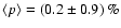 ,
provides a measurement
of the maximum instrumental linear polarization
affecting our polarization fits,
,
provides a measurement
of the maximum instrumental linear polarization
affecting our polarization fits,
 ,
which we consider
negligible for the purposes of our data analysis.
The fact that
,
which we consider
negligible for the purposes of our data analysis.
The fact that
 is of similar
magnitude than
indicates that, as
for the total flux density measurements, our
polarization accuracy is most likely limited
by the statistical uncertainties induced by the
small and rapid atmospheric fluctuations.
is of similar
magnitude than
indicates that, as
for the total flux density measurements, our
polarization accuracy is most likely limited
by the statistical uncertainties induced by the
small and rapid atmospheric fluctuations.
Such uncertainties are computed from the linear
polarization fits.
In the case of 0716+714, for time periods
 h, they lie in the range 1.2 %
to 3.4 % for p and between 0.06 Jy and
0.12 Jy for P (see Sect. 3.2).
The additional error (a 5% of the total flux
density) coming from the inaccuracy on the
absolute flux density scaling, has been added in
quadrature wherever it was necessary for the final
P results; i.e. only for non-relative variability
results.
In such cases, we explicitly indicate that this
additional error was added.
h, they lie in the range 1.2 %
to 3.4 % for p and between 0.06 Jy and
0.12 Jy for P (see Sect. 3.2).
The additional error (a 5% of the total flux
density) coming from the inaccuracy on the
absolute flux density scaling, has been added in
quadrature wherever it was necessary for the final
P results; i.e. only for non-relative variability
results.
In such cases, we explicitly indicate that this
additional error was added.
The accuracy of our polarization angle
estimates is better tested on sources with large
linear polarization fraction, which should show
large modulation amplitudes in functions
(2) and (3), and hence should
allow for a more accurate measurement of  .
Among our observed sources, 0716+714 was the most
suitable one for such test, since it showed the
highest polarization degree
(see Sect. 3) and was better time sampled.
The two independent fits of functions (2) and
(3) to the 0716+714 data, over ten different
time ranges of h (Sect. 3.2),
showed an internal consistency of the estimates to a precision better than
.
Among our observed sources, 0716+714 was the most
suitable one for such test, since it showed the
highest polarization degree
(see Sect. 3) and was better time sampled.
The two independent fits of functions (2) and
(3) to the 0716+714 data, over ten different
time ranges of h (Sect. 3.2),
showed an internal consistency of the estimates to a precision better than
 .
This demonstrates the
accuracy of equations (2), (3)
and (4) and the good orthogonality
of the signals recorded by receivers A100 and B100.
However, the statistical uncertainties on the
determination of
fail to be better than
.
This demonstrates the
accuracy of equations (2), (3)
and (4) and the good orthogonality
of the signals recorded by receivers A100 and B100.
However, the statistical uncertainties on the
determination of
fail to be better than
 even for
the polarization fits to the 0716+714 data over
the whole observing time.
Also for 0716+714, these uncertainties range
between
even for
the polarization fits to the 0716+714 data over
the whole observing time.
Also for 0716+714, these uncertainties range
between
 and
and  for the
ten time spans with h
(Sect. 3.2).
for the
ten time spans with h
(Sect. 3.2).
![\begin{figure}
\par\includegraphics[width=9cm,clip]{4649fig1.eps}
\end{figure}](/articles/aa/full/2006/34/aa4649-05/img82.gif) |
Figure 1:
Calibrated measurements of
 and
and
 for 0716+714 vs. time during 2003 November 10 to 16.
The sinusoidal pattern is due to source polarization
(see the text).
for 0716+714 vs. time during 2003 November 10 to 16.
The sinusoidal pattern is due to source polarization
(see the text). |
| Open with DEXTER | |
Note that the accuracy of absolute polarization
angle measurements obtained from A100 and B100
data is driven by the accuracy of the orientation
of their polarization axes (see Appendix A and
Thum et al. 2000).
Such orientations were calibrated with an accuracy
of
 (Clemens Thum, private
communication), which is therefore the better absolute
polarization angle accuracy achievable with the A100 and B100 receivers.
A corresponding error of
(Clemens Thum, private
communication), which is therefore the better absolute
polarization angle accuracy achievable with the A100 and B100 receivers.
A corresponding error of  has been added
quadratically to the
statistical uncertainties
of our measurements obtained for the whole observing
time range, but not to those computed for shorter time
spans - which are aimed at relative variability
analyses -.
has been added
quadratically to the
statistical uncertainties
of our measurements obtained for the whole observing
time range, but not to those computed for shorter time
spans - which are aimed at relative variability
analyses -.
In Fig. 1 we present plots of the resulting calibrated
responses of receivers A100 and B100 to the 0716+714 emission
during November 11 to 17. The curves show a remarkable increase of
 Jy in
and
during
November 10 to 14 together with a large amplitude sinusoidal
modulation, which has a characteristic periodicity of 12 h
and has a phase difference of
Jy in
and
during
November 10 to 14 together with a large amplitude sinusoidal
modulation, which has a characteristic periodicity of 12 h
and has a phase difference of  rad between the
and
patterns.
The main contribution to this modulation is explained by
the right-hand terms of expressions (2) and (3), which are significative when the source is
highly linearly polarized.
Following (2) and (3), the linear
polarization flux density of 0716+714 can be estimated
from the amplitudes of the modulations of the
and
curves, which lie in the range
rad between the
and
patterns.
The main contribution to this modulation is explained by
the right-hand terms of expressions (2) and (3), which are significative when the source is
highly linearly polarized.
Following (2) and (3), the linear
polarization flux density of 0716+714 can be estimated
from the amplitudes of the modulations of the
and
curves, which lie in the range
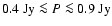 .
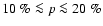
Hence, the curves in Fig. 1
represent the first evidence of a high degree of linear
polarization (
.
Hence, the curves in Fig. 1
represent the first evidence of a high degree of linear
polarization (
 )
in 0716+714 at 86 GHz.
As far as we know, such a high linear polarization
was never observed before in the integrated emission
of 0716+714 in any radio to mm band.
)
in 0716+714 at 86 GHz.
As far as we know, such a high linear polarization
was never observed before in the integrated emission
of 0716+714 in any radio to mm band.
In Fig. 2 we show the calibrated response of B230 to
the 0716+714 emission during November 10 to 15.
The larger measurement uncertainties at 229 GHz,
which are typically 18%, do not allow us to detect
IDV with amplitude lower than this level.
Therefore, we are able to determine only the basic
emission properties at this frequency.
Since at 229 GHz 0716+714 does not show the expected
12 h periodic polarization modulation, then, within the
errors, the response of B230 is a valid measurement of the source
total flux density (S229).
![\begin{figure}
\par\includegraphics[width=9cm,clip]{4649fig2.eps}
\end{figure}](/articles/aa/full/2006/34/aa4649-05/img88.gif) |
Figure 2:
Calibrated measurements of
 for
0716+714, 0836+710 and
1928+738 during 2003 November 10 to 15.
The dashed line on the top inset represents the best
linear fit to the 0716+714 light curve.
for
0716+714, 0836+710 and
1928+738 during 2003 November 10 to 15.
The dashed line on the top inset represents the best
linear fit to the 0716+714 light curve. |
| Open with DEXTER | |
Accurate measurements of the 86 GHz flux densities (S86(i))
were obtained by averaging together
and
(see Appendix A).
The resulting evolution of
 during the time range
of our observations of 0716+714 is presented in Fig. 3
together with the light curves of the non-IDV sources 0836+710
and 1928+738. The latter demonstrate the accuracy of our
calibration, which provided flux density measurements characterised
by an rms
during the time range
of our observations of 0716+714 is presented in Fig. 3
together with the light curves of the non-IDV sources 0836+710
and 1928+738. The latter demonstrate the accuracy of our
calibration, which provided flux density measurements characterised
by an rms
 %. This represents an unprecedented
stability for 86 GHz measurements with the IRAM 30 m telescope.
%. This represents an unprecedented
stability for 86 GHz measurements with the IRAM 30 m telescope.
![\begin{figure}
\par\includegraphics[width=9cm,clip]{4649fig3.eps}
\end{figure}](/articles/aa/full/2006/34/aa4649-05/img91.gif) |
Figure 3: Calibrated 86 GHz light curves of 0716+714, 0836+710 and 1928+738 during 2003 November 10 to 16. The dashed line on the top inset represents the best linear fit to the 0716+714 flux density evolution during 2003 November 10 to 15. |
| Open with DEXTER | |
The variability of 0716+714 at 86 GHz appears to be dominated
by a monotonous linear increase from
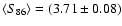 Jy
during November 10 to 11 to
Jy
during November 10 to 11 to
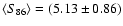 Jy during
November 15 (with
Jy during
November 15 (with
 denoting averaging in time).
During the 5 h of data obtained on November 16, the
source displayed a similar mean flux density of
denoting averaging in time).
During the 5 h of data obtained on November 16, the
source displayed a similar mean flux density of
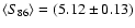 Jy.
The linear fit of the light curve from days 10 to 15
(Fig. 3) gives an increasing rate
(
Jy.
The linear fit of the light curve from days 10 to 15
(Fig. 3) gives an increasing rate
(
 )
of
)
of
 %/day.
The fit performed to the 229 GHz light curve gives
%/day.
The fit performed to the 229 GHz light curve gives
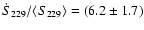 %/day, which shows a
similar trend at both observing frequencies. This suggests that
the variability at both 86 GHz and 229 GHz originates
from the same region of the source and the same physical process.
%/day, which shows a
similar trend at both observing frequencies. This suggests that
the variability at both 86 GHz and 229 GHz originates
from the same region of the source and the same physical process.
To characterise the flux density variability of each
source we used the statistical formulation described in
Quirrenbach et al. (2000) and Kraus et al.
(2003).
In particular, we made use of the modulation index m, the
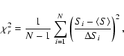
variability amplitude Y, the reduced chi-squared
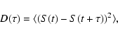
 and the structure function
  .
The
corresponding definitions are summarised in Appendix B.
.
The
corresponding definitions are summarised in Appendix B.
The computed statistical parameters for 0716+714 and the secondary calibrators are listed in Table 3 for both the 86 GHz and the 229 GHz data set. The computation of the variability amplitude Y was performed only for those sources that passed the chi-squared test (variable with significance level >99.9%). As can be seen in the table, only 0716+714 showed such significant variability (at 86 GHz, but not at 229 GHz due to the larger uncertainties at that frequency).
Although 1642+690 formally did not pass this test, it displayed
larger values of m and
than the remaining
calibrators at both 86 GHz and 229 GHz (see Table 3),
suggesting a weaker variability.
In fact, its 86 GHz light curve (frequency at which
the variability analysis is more accurate) is variable at
confidence level >95%.
Based on this evidence, we excluded 1642+690 as secondary
calibrator from the 86 GHz and 229 GHz data reduction.
Table 3: Statistical parameters characterising the variability of 0716+714 and the secondary calibrators during 2003 November 10 to 16.
The structure function
for 0716+714 at 86 GHz is
shown in Fig. 4. The shape of this function provides
the variability type classification of the observed sources
(Heeschen et al. 1987; Kraus et al. 2003).
The lack of pronounced maxima and of a saturation point in on time lags shorter than two days allows us to classify
0716+714 as an IDV source of type I during the time range
of our observations at 86 GHz.
The local maximum appearing at a time lag of 4 days
characterises the time-scale of the monotonic increase of the
flux density S86.
In agreement with this, and based on the same data set,
Fuhrmann et al. (in prep.) report, from a more sophisticated
estimate, a time-scale of
3.83+0.14-0.15 days.
![\begin{figure}
\par\includegraphics[width=8.1cm,clip]{4649fig4.eps}
\end{figure}](/articles/aa/full/2006/34/aa4649-05/img104.gif) |
Figure 4:
function for 0716+714 at 86 GHz. Since the
data are unevenly sampled, we derived
using
an interpolation procedure. A minimal interpolation
interval of
 h (3 to 5 times larger than the
typical S86 sampling time-range) was chosen. To
assess the errors caused by the interpolation,
was derived twice, first by starting at the beginning of
the time series and second by proceeding backwards. h (3 to 5 times larger than the
typical S86 sampling time-range) was chosen. To
assess the errors caused by the interpolation,
was derived twice, first by starting at the beginning of
the time series and second by proceeding backwards. |
| Open with DEXTER | |
The 86 GHz polarization estimates were obtained by fitting
the functions (2) and (3), which relate
directly the amplitudes and phases of such polarization patterns
to the linearly polarized flux density P and electric vector
position angle
of the observed source, respectively.
The fits performed for 0716+714 for 12 h time bins (with
a minimum of ten points per fit) are shown in Fig. 5.
This time binning was chosen as the optimum to provide more than
one P and
measurement per day and the lowest
possible uncertainties in their estimate.
Polarization fits for
 h time bins and for
the entire time range of the observations were also performed for
both 0716+714 and the secondary calibrators
(Fig. 6, Tables 4 and 5).
h time bins and for
the entire time range of the observations were also performed for
both 0716+714 and the secondary calibrators
(Fig. 6, Tables 4 and 5).
![\begin{figure}
\par\includegraphics[width=18cm,clip]{4649fig5.eps}
\end{figure}](/articles/aa/full/2006/34/aa4649-05/img107.gif) |
Figure 5:
Plots of the fits of functions (2) and
(3) to the 86 GHz data of 0716+714. Each
plot represents a time bin
 12 h of observing time
(labelled within each of them) with a minimum of ten data
points. The time spans, ordered from top to bottom and
from left to right, cover the whole observing time.
The whole data set has been plotted together in the
right-bottom plot. The sinusoidal lines represent the
independent non-linear least squares fits of functions (2) and (3).
The resulting averaged P and
variables are
given within each corresponding plot.
Errors were originallycomputed as 1-
uncertainties from the fits.
For the right-bottom plot, the errors from
the absolute total flux density and polarization angle
uncertainties (see Sect. 2) have been taken
int account (added in quadrature). 12 h of observing time
(labelled within each of them) with a minimum of ten data
points. The time spans, ordered from top to bottom and
from left to right, cover the whole observing time.
The whole data set has been plotted together in the
right-bottom plot. The sinusoidal lines represent the
independent non-linear least squares fits of functions (2) and (3).
The resulting averaged P and
variables are
given within each corresponding plot.
Errors were originallycomputed as 1-
uncertainties from the fits.
For the right-bottom plot, the errors from
the absolute total flux density and polarization angle
uncertainties (see Sect. 2) have been taken
int account (added in quadrature). |
| Open with DEXTER | |
The fits presented in Fig. 5 confirm the
previously mentioned high polarization level of 0716+714
at 86 GHz.
The average polarization properties of the source
(during our observations) were
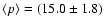 %, or
%, or
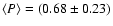 Jy, and
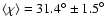 (Table 4),
where the errors of
(Table 4),
where the errors of
 and
and
 take into account
those from the absolute total flux density and polarization
angle uncertainties, respectively (see Sect. 2).
Such a high polarization degree is rather unusual for AGN at
centimetre wavelengths, for which p>10% is rarely
observed even during flaring states (e.g. Aller et al.
1999) and typically
take into account
those from the absolute total flux density and polarization
angle uncertainties, respectively (see Sect. 2).
Such a high polarization degree is rather unusual for AGN at
centimetre wavelengths, for which p>10% is rarely
observed even during flaring states (e.g. Aller et al.
1999) and typically
 %.
Synchrotron self-absorption, usually dominating at low
centimetre radio frequencies, can reduce p (e.g. Pacholczyk 1970). However, low values
of polarization degree are observed at centimetre
wavelengths even for optically thin sources.
Numerical simulations show that, in order to explain
these low levels of polarization in compact radio sources,
a large fraction of the magnetic field (typically
50%-70%) should be disordered in direction
(e.g. Gómez, Alberdi & Marcaide 1993).
The 15% polarization degree detected in 0716+714 might
indicate a high level of magnetic field alignment
in the region from which the 86 GHz emission originated.
%.
Synchrotron self-absorption, usually dominating at low
centimetre radio frequencies, can reduce p (e.g. Pacholczyk 1970). However, low values
of polarization degree are observed at centimetre
wavelengths even for optically thin sources.
Numerical simulations show that, in order to explain
these low levels of polarization in compact radio sources,
a large fraction of the magnetic field (typically
50%-70%) should be disordered in direction
(e.g. Gómez, Alberdi & Marcaide 1993).
The 15% polarization degree detected in 0716+714 might
indicate a high level of magnetic field alignment
in the region from which the 86 GHz emission originated.
In addition, one of the six observed AGN calibrators,
0212+735, also displays a
polarization degree p>10% and 0633+734 and
1803+784 show  %.
These values are still high when compared with the typically
observed polarization degrees at centimetre wavelengths.
The fact that, at 86 GHz, more than 50% of the observed
AGN display larger polarization degrees than those typically
measured at centimetre wavelengths might suggest that the
polarization degree in AGN increases with frequency.
This would indicate higher ordering of the magnetic
fields in the deeper regions of their jets observed in the
millimetre bands respect to centimetre wavelengths.
However, it is clear that our sampled set of AGN is not
statistically significant enough to strongly support
this hypothesis.
The millimetre polarization survey performed
by Thum et al. (in prep.) over more than 70 AGN
during the summer of 2006 will certainly improve the
statistics.
%.
These values are still high when compared with the typically
observed polarization degrees at centimetre wavelengths.
The fact that, at 86 GHz, more than 50% of the observed
AGN display larger polarization degrees than those typically
measured at centimetre wavelengths might suggest that the
polarization degree in AGN increases with frequency.
This would indicate higher ordering of the magnetic
fields in the deeper regions of their jets observed in the
millimetre bands respect to centimetre wavelengths.
However, it is clear that our sampled set of AGN is not
statistically significant enough to strongly support
this hypothesis.
The millimetre polarization survey performed
by Thum et al. (in prep.) over more than 70 AGN
during the summer of 2006 will certainly improve the
statistics.
Inspection of Fig. 5 indicates time-dependent
changes in both the amplitude and the phase of the fitted
functions, suggesting that the linear polarization
of 0716+714 varied along our observations.
The P estimates, for both 0716+714 and the secondary
calibrators, are presented as a function of time
in Fig. 7, while the
evolution
for 0716+714 only is shown in Fig. 8.
Due to the much lower polarization degree of the calibrators,
their polarization properties were optimally fitted with
time bins of
 h.
This provided one polarization measurement per day to test the
stability of the secondary calibrators and it also decreased
the fitting errors compared to shorter time-binnings.
To allow for a better comparison with the calibrators,
the 0716+714 data were also fitted using a
h time binning (Fig. 7,
Fig. 8 and Table 5).
h.
This provided one polarization measurement per day to test the
stability of the secondary calibrators and it also decreased
the fitting errors compared to shorter time-binnings.
To allow for a better comparison with the calibrators,
the 0716+714 data were also fitted using a
h time binning (Fig. 7,
Fig. 8 and Table 5).
![\begin{figure*}
\par\includegraphics[width=18cm,clip]{4649fig6.eps}
\end{figure*}](/articles/aa/full/2006/34/aa4649-05/img117.gif) |
Figure 6:
86 GHz polarization patterns of the secondary
calibrators. For the sake of clarity, a shift
of rad was added to function (3) to match
function (2), i.e.
 (see Sect. 2.3).
For each source, the data from the whole observing time-range
is presented.
The sinusoidal lines represent the non-linear least squares
fits to the data.
The resulting averaged P and
variables are
given within each corresponding plot.
The errors presented on each plot were computed
by adding in quadrature the 1-
uncertainties from the fits and the errors from
the absolute total flux density and polarization angle
uncertainties (see Sect. 2).
(see Sect. 2.3).
For each source, the data from the whole observing time-range
is presented.
The sinusoidal lines represent the non-linear least squares
fits to the data.
The resulting averaged P and
variables are
given within each corresponding plot.
The errors presented on each plot were computed
by adding in quadrature the 1-
uncertainties from the fits and the errors from
the absolute total flux density and polarization angle
uncertainties (see Sect. 2). |
| Open with DEXTER | |
While the secondary calibrators remained stable in polarization
within the errors, 0716+714 displayed polarization
variability during November 11 and 14.
To quantify this variability, we performed
a statistical analysis similar to the one presented in Sect. 3.1.
Due to the much weaker polarization of the secondary calibrators
compared to 0716+714, the errors of their P and especially
their
estimates are much larger than for 0716+714.
Hence, in principle, it would not be reasonable to calculate mP,  ,
YP
and
,
YP
and  since they do
not take into account the uncertainties on the measurements
and they would not provide reliable variability results.
However, the mean, the standard deviation and the reduced chi-squares
of both the P and
distributions can still provide useful
statistical information.
These magnitudes are summarised in Table 5.
None of the sources analysed passed the chi-squared test
neither for P nor for .
However, 0716+714
displayed relatively large values of
since they do
not take into account the uncertainties on the measurements
and they would not provide reliable variability results.
However, the mean, the standard deviation and the reduced chi-squares
of both the P and
distributions can still provide useful
statistical information.
These magnitudes are summarised in Table 5.
None of the sources analysed passed the chi-squared test
neither for P nor for .
However, 0716+714
displayed relatively large values of
 and
and
 ,
with corresponding variability
significance levels
,
with corresponding variability
significance levels
 %.
Hence, for the particular case of 0716+714 and given the
relatively large significance of its polarization variability,
it makes sense to compute both mP=15% and
%.
Hence, for the particular case of 0716+714 and given the
relatively large significance of its polarization variability,
it makes sense to compute both mP=15% and
 ,
which are attributed to the source behaviour during the first
four observing days (Figs. 7 and 8).
,
which are attributed to the source behaviour during the first
four observing days (Figs. 7 and 8).
Table 4: Average 86 GHz polarization properties of 0716+714 and the secondary calibrators during 2003 November 10 to 16.
Table 5: Statistical parameters characterising the 86 GHz polarization variability of 0716+714 and the secondary calibrators, but 1928+738, during 2003 November 10-16.
![\begin{figure}
\par\includegraphics[width=8.1cm,clip]{4649fig7.eps}
\end{figure}](/articles/aa/full/2006/34/aa4649-05/img149.gif) |
Figure 7:
86 GHz P curves for 0716+714, 0836+710 and
1803+784. Time bins of <24 h were used for
all the sources. For 0716+714 the results for time
bins
 h are also presented. Horizontal bars
symbolise the time range over which each estimate of P was
computed. h are also presented. Horizontal bars
symbolise the time range over which each estimate of P was
computed. |
| Open with DEXTER | |
![\begin{figure}
\par\includegraphics[width=8.2cm,clip]{4649fig8.eps}
\end{figure}](/articles/aa/full/2006/34/aa4649-05/img150.gif) |
Figure 8:
86 GHz polarization angle vs. time for 0716+714.
The results obtained for time bins of both
<24 h and
12 h are presented.
Horizontal bars symbolise the time range over which each
estimate was computed. For the sake of clarity,
the
time series of the calibrators (which are all
constant within their corresponding errors) have not been
plotted due to their large uncertainties, typically of
15 -20. -20. |
| Open with DEXTER | |
The amount of P and
variability of 0716+714 between
each pair of adjacent measurements of these variables was
characterised through their fractional variability amplitudes:
 (with
i=1,2,...,10 for the 0716+714
polarization measurements performed with a time binning
(with
i=1,2,...,10 for the 0716+714
polarization measurements performed with a time binning
 h) denotes for the
interval over which each one of the polarization fits
was performed and
h) denotes for the
interval over which each one of the polarization fits
was performed and
 symbolises the time
interval between each pair of adjacent polarization measurements.
We considered that an intra-day polarization variation
event is significant when either VP or
symbolises the time
interval between each pair of adjacent polarization measurements.
We considered that an intra-day polarization variation
event is significant when either VP or  is larger than its corresponding uncertainties
computed by propagating the errors of P and .
There is only one time interval (
is larger than its corresponding uncertainties
computed by propagating the errors of P and .
There is only one time interval (
 )
for which
this condition is fulfilled.
is a time
interval of 24 h on November 13-14, for which both
)
for which
this condition is fulfilled.
is a time
interval of 24 h on November 13-14, for which both
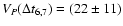 % and
% and
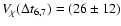 % show a
  variation in P and ,
respectively (see Fig. 9).
Hence, this simple analysis provided indications of IDV on the
polarized emission of 0716+714 during our observations.
Nevertheless, this statement should not be taken as a
strong evidence of polarization IDV, as no
variation in P and ,
respectively (see Fig. 9).
Hence, this simple analysis provided indications of IDV on the
polarized emission of 0716+714 during our observations.
Nevertheless, this statement should not be taken as a
strong evidence of polarization IDV, as no  IDV event has been detected.
A future dedicated millimetre monitoring campaign, optimised
for high time sampling and high polarization sensitivity,
will be necessary to confirm and clarify whether
0716+714 (or any other AGN) is variable in polarization on
time-scales of 24 h.
IDV event has been detected.
A future dedicated millimetre monitoring campaign, optimised
for high time sampling and high polarization sensitivity,
will be necessary to confirm and clarify whether
0716+714 (or any other AGN) is variable in polarization on
time-scales of 24 h.
![\begin{figure}
\par\includegraphics[width=8.2cm,clip]{4649fig9.eps}
\end{figure}](/articles/aa/full/2006/34/aa4649-05/img161.gif) |
Figure 9:
Amplitude of fractional polarization variability,
as a function of time. The vertical bars represent
the VP and
propagated errors whereas
the horizontal bars symbolise the maximum possible
time range over which the variability took place.
See the text for definitions. |
| Open with DEXTER | |
The millimetre data presented here contributed to the
assembling of the broad-band spectrum (from radio to
-rays) of 0716+714 during November 10 to 16,
2003 presented by Ostorero et al. (2006).
The spectrum was inverted between the cm- and mm-bands.
Its turnover frequency ( ,
at which the synchrotron
spectrum peaks) was located at
,
at which the synchrotron
spectrum peaks) was located at
 GHz.
Between 86 GHz and 667 GHz the spectrum can be fitted by a single
power law with spectral index
GHz.
Between 86 GHz and 667 GHz the spectrum can be fitted by a single
power law with spectral index
 (where
 and
and  denotes the observing
frequencies within this spectral range).
denotes the observing
frequencies within this spectral range).
At 86 GHz, the total flux density of the source (Sect. 3.1)
ranged from
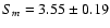 Jy at the 10.88 UT days of
November 2003 to
Jy at the 10.88 UT days of
November 2003 to
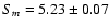 Jy at the 15.00 UT days
of November 2003.
The larger total flux density of the source at 86 GHz
compared to that at 229 GHz, (Figs. 2 and 3)
shows that the source synchrotron spectrum was optically thin
between these two frequencies during the whole time range of
our observations.
To attempt to characterise the source spectral evolution, we have
computed the spectral index for each pair of S86(i) and
S229(i), where i is the index defining each one of the
simultaneous 86 GHz and 229 GHz measurements.
The resulting
Jy at the 15.00 UT days
of November 2003.
The larger total flux density of the source at 86 GHz
compared to that at 229 GHz, (Figs. 2 and 3)
shows that the source synchrotron spectrum was optically thin
between these two frequencies during the whole time range of
our observations.
To attempt to characterise the source spectral evolution, we have
computed the spectral index for each pair of S86(i) and
S229(i), where i is the index defining each one of the
simultaneous 86 GHz and 229 GHz measurements.
The resulting
 evolution (shown in Fig. 10) is consistent with a decreasing pattern (spectral
softening) with constant rate
evolution (shown in Fig. 10) is consistent with a decreasing pattern (spectral
softening) with constant rate
 and average
 from the 10.88 to the 15.00 U.T. days of November 2003.
However, the computed
from the 10.88 to the 15.00 U.T. days of November 2003.
However, the computed
 is not
statistically significant and the possible spectral change of
0716+714 needs to be tested through more accurate spectral
index data.
is not
statistically significant and the possible spectral change of
0716+714 needs to be tested through more accurate spectral
index data.
![\begin{figure}
\par\includegraphics[width=8.2cm,clip]{4649fig10.eps}
\end{figure}](/articles/aa/full/2006/34/aa4649-05/img172.gif) |
Figure 10:
Evolution of the spectral index
in
0716+714.
The absolute total flux density calibration
errors of S86 and S229 (see Sect. 2)
were taken into account to compute those of
.
The dashed line represents the best linear
fit to the data, which is consistent with a
pattern with a rate
and average
. |
| Open with DEXTER | |
Given the known frequency dependence for weak ISS, it is rather unlikely that the Y=34% amplitude inter-day variability reported at 86 GHz is caused by this extrinsic effect. As outlined in Sect. 1, such large variability in the mm-bands can not be reproduced by the standard ISS models (e.g. Beckert et al. 2002). Fuhrmann et al. (in prep.) perform a more detailed variability study combining all the available simultaneous data from 5 GHz to 667 GHz, and show that the inter-day variations shown in this paper contradict the predictions of such models. We should hence attribute the large amplitude 86 GHz variability of 0716+714 to intrinsic causes.
Hence, the high amplitude inter-day variability reported by Ostorero et al. (2006) at 32 GHz and 37 GHz, which well matches with the millimetre behaviour shown in this paper, was most likely produced in the source itself and not by ISS. Ostorero et al. (2006) also report on the rapid IDV in the optical range observed during the time range of our IRAM 30 m observations. Although 0716+714 did not show evidence of simultaneous radio or mm and optical IDV-time-scale transitions, as during previous monitoring campaigns (Quirrenbach et al. 1991), this can not be taken as an argument in favour of the extrinsic origin of the variability. It indicates only that, during our observations, the radio-mm emission was radiated from a different region, or through a different mechanism, than that producing the optical emission.
Under the assumption that the main component of the
mm-variability is intrinsic to the source and via the causality
argument, it is possible to estimate some of the physical conditions
governing the source.
This can be performed by modelling it as a relativistically moving
homogeneous sphere (e.g. Marscher et al. 1979;
Ghisellini et al. 1993).
Under these assumptions, the intrinsic brightness temperature
of the emitting region at the turnover frequency (at which the spectral index is zero, by definition) can be computed
from its variability time scale as:
is in GHz. z is the redshift of the source,  is an equivalent
Doppler factor and
is an equivalent
Doppler factor and
 is the variability time scale
in days and
is the variability time scale
in days and  is the source luminosity distance in Gpc.
In this paper, we adopt
z=0.3 (the lower limit for the redshift of 0716+714, see e.g.
Sect. 1 and Wagner et al. 1996), a Hubble constant
H0=72 km s-1 Mpc-1 and a
Friedmann- Robertson-Walker cosmology with
is the source luminosity distance in Gpc.
In this paper, we adopt
z=0.3 (the lower limit for the redshift of 0716+714, see e.g.
Sect. 1 and Wagner et al. 1996), a Hubble constant
H0=72 km s-1 Mpc-1 and a
Friedmann- Robertson-Walker cosmology with
 and
and
 .
Within these assumptions,
.
Within these assumptions,
 Gpc.
Gpc.
Our 86 GHz observations provide us the values of
Sm=5.23 Jy,
 Jy,
Jy,
 Jy,
Jy,
 days and
 days.
The only remaining variable in expression (7) which can not
be directly observed is .
By assuming
a non-moving source, expression (7) gives us the
apparent brightness temperature
days.
The only remaining variable in expression (7) which can not
be directly observed is .
By assuming
a non-moving source, expression (7) gives us the
apparent brightness temperature
 K at z=0.3,
which exceeds by more than two orders of magnitude the IC-limit
K at z=0.3,
which exceeds by more than two orders of magnitude the IC-limit
 K (Kellermann & Pauliny-Toth
1969). Hence,
K (Kellermann & Pauliny-Toth
1969). Hence,
 sets a lower limit to the
Doppler factor of the emitting region, which should then be
sets a lower limit to the
Doppler factor of the emitting region, which should then be
 .
Note that a more accurate limit for
(of
.
Note that a more accurate limit for
(of
 K) was computed by Readhead (1994)
(see also Kellermann 2003). To avoid the violation of the
latter,
K) was computed by Readhead (1994)
(see also Kellermann 2003). To avoid the violation of the
latter,
 is required.
The latter constraint (
), together with
expression (8), allows us to estimate an upper limit for
the size of the emitting region responsible for the variability
during our observations, which should be
 mas.
Obviously,
mas.
Obviously,
 is also an upper limit for the
maximum size of such region obtained from
.
is also an upper limit for the
maximum size of such region obtained from
.
It should be stressed that
does not account
for the size of the whole source, but only for the region responsible
for the rapid variability, which in the case of 0716+714 has been
associated with the VLBI core component of its relativistic
jet (Bach et al. 2006).
An independent constraint on the size of the variability
region can be obtained from the 86 GHz VLBI observations of
0716+714 performed by Bach et al. (2006) in April 2003.
A Gaussian model fit of their resulting image gives a FWHM size
of the 86 GHz VLBI core of 0.014 mas, which is much lower
than the minimum beam size of VLBI observations at
such frequency (
 mas; e.g. Agudo et al. 2005).
This gives us
mas; e.g. Agudo et al. 2005).
This gives us
 mas, which is in agreement
with our estimate of
.
mas, which is in agreement
with our estimate of
.
We will hence assume hereafter that the true angular size of the
rapid variability region is
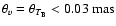 .
.
It is also possible to compare the expected and the observed
first order self-Compton -ray flux density to constrain the
IC Doppler factor (
 )
of the source
(Marscher 1983 and Ghisellini et al.
1993).
is defined as:
)
of the source
(Marscher 1983 and Ghisellini et al.
1993).
is defined as:
 is the spectral index of the optically thin
synchrotron spectrum (
is the spectral index of the optically thin
synchrotron spectrum (
 has been adopted here),
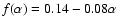 (Ghisellini et al.
1993 and references therein),
(Ghisellini et al.
1993 and references therein),  is the upper
frequency cut-off of the synchrotron spectrum in GHz,
is the upper
frequency cut-off of the synchrotron spectrum in GHz,
 is the -ray energy in keV and
 is the
measured -ray flux at
in Jy.
,
in GHz, is the most poorly
known variable among those in Eq. (9).
However, this problem is overcome
by the fact that
is the
measured -ray flux at
in Jy.
,
in GHz, is the most poorly
known variable among those in Eq. (9).
However, this problem is overcome
by the fact that
 is a weak function of ,
which is contained within a logarithmic factor. Here, we have
assumed
is a weak function of ,
which is contained within a logarithmic factor. Here, we have
assumed
 GHz
(Biermann & Strittmatter 1987).
Implicit to Eq. (9) is the assumption that the
electrons radiating the synchrotron emission have a power-law
energy distribution (
GHz
(Biermann & Strittmatter 1987).
Implicit to Eq. (9) is the assumption that the
electrons radiating the synchrotron emission have a power-law
energy distribution (
 ,
with
,
with
 )
and that the
magnetic field is tangled in the rest frame of the
emitting plasma.
)
and that the
magnetic field is tangled in the rest frame of the
emitting plasma.
By taking into account the dependence of
 on
in (9),
can be written
as:
on
in (9),
can be written
as:
 .
.
The results of the simultaneous INTEGRAL soft -ray observations
of 0716+714 reported by Ostorero et al. (2006)
(
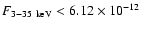 erg cm-2 s-1,
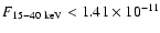 erg cm-2 s-1,
 erg cm-2 s-1 and
 erg cm-2 s-1;
see also Table 6 for the corresponding flux densities in
Jy), together with expression (10), allow us to set new
constraints on the Doppler factor of 0716+714
during our observations.
Assuming
days as in Sect. 4.3,
we derive lower limits of
erg cm-2 s-1;
see also Table 6 for the corresponding flux densities in
Jy), together with expression (10), allow us to set new
constraints on the Doppler factor of 0716+714
during our observations.
Assuming
days as in Sect. 4.3,
we derive lower limits of
 ,
,
 ,
,
 and
and
 from the
upper limits of the flux densities of the source at 8 keV,
23 keV, 63 keV and 141 keV, respectively.
from the
upper limits of the flux densities of the source at 8 keV,
23 keV, 63 keV and 141 keV, respectively.
It is worth to note that, for
,
expression (10) is a weak function of the redshift and the luminosity
distance of the source (
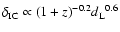 ). Hence, the constraint on the Doppler
factor of the source provided by (10),
). Hence, the constraint on the Doppler
factor of the source provided by (10),
 ,
is more robust than those
derived from expression (7) and the limits for
,
is more robust than those
derived from expression (7) and the limits for
 (Sect. 4.3).
Table 6: Physical parameter estimates. See the text for definitions.
We have presented the results from millimetre observations of 0716+714, which were performed on 2003 November 10 to 18 with the IRAM 30 m telescope. Our observation strategy, based on the rapid time sampling of both the target source and the calibrators, enabled us to reach a relative calibration accuracy of 1.2% at 86 GHz, which demonstrates the good performance of this telescope and its ability for future accurate IDV studies in the millimetre range.
During our first four observing days, the source displayed large amplitude (Y=34%) and monotonous inter-day variability at 86 GHz. As such large amplitude variability is not expected to be produced by standard ISS at mm wavelengths (Rickett et al. 1995), this variation should be considered as intrinsic to the source and not due to the influence of the interstellar medium. The similar 32 GHz and 37 GHz behaviour reported by Ostorero et al. (2006) during the same observing time range could hence be explained by intrinsic causes also.
Ostorero et al. (2006) also report clear evidence of IDV in the optical range, which is not matched either in the mm or in the cm bands (see also Fuhrmann et al. in prep.). This indicates that the radio-mm emitting region was located in a different region than the optical one or that their radiation behaviours were driven by different physical processes during our observations.
We have reported an unusually large linear
polarization degree
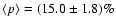 of 0716+714 at 86 GHz, which suggests a large level
of magnetic field alignment.
At such frequency, linear polarization inter-day
variability, with significance level
of 0716+714 at 86 GHz, which suggests a large level
of magnetic field alignment.
At such frequency, linear polarization inter-day
variability, with significance level
 ;
% and
,
was observed during the first four observing days.
We have also shown
evidence of simultaneous
polarization flux density and polarization angle IDV within
a time 24 h.
If such rapid polarization variations that are uncorrelated
with the total flux density variability are confirmed by future
observations, then equally rapid changes of the magnetic field
configuration of the source or changes of opacity around would be required to explain the phenomenon.
In both cases, inhomogeneous models would probably
have to be invoked.
;
% and
,
was observed during the first four observing days.
We have also shown
evidence of simultaneous
polarization flux density and polarization angle IDV within
a time 24 h.
If such rapid polarization variations that are uncorrelated
with the total flux density variability are confirmed by future
observations, then equally rapid changes of the magnetic field
configuration of the source or changes of opacity around would be required to explain the phenomenon.
In both cases, inhomogeneous models would probably
have to be invoked.
The synchrotron spectrum of 0716+714 peaked at
GHz during 2003 November 10 to 15
(Ostorero et al. 2006), and showed
an optically thin spectral index
between 86 GHz and 229 GHz. The apparent brightness temperature
derived from our 86 GHz light curve,
K for a redshift z=0.3, exceeds, at least by
two orders of magnitude, the IC-limit of
 K
(Kellemann & Pauliny-Toth 1969; Readhead 1994;
Kellermann 2003).
This mismatch can be explained by the relativistic motion or
expansion of the source with a minimum Doppler factor
.
The upper limits from the soft -ray simultaneous
INTEGRAL observations in the 3 keV to 200 keV energy range
enabled us to compute an independent and more robust limit
for the source Doppler factor,
K
(Kellemann & Pauliny-Toth 1969; Readhead 1994;
Kellermann 2003).
This mismatch can be explained by the relativistic motion or
expansion of the source with a minimum Doppler factor
.
The upper limits from the soft -ray simultaneous
INTEGRAL observations in the 3 keV to 200 keV energy range
enabled us to compute an independent and more robust limit
for the source Doppler factor,
 .
This limit is consistent with previous estimates of
the Doppler factor of 0716+714 measured from the kinematics
of VLBI-scale jet features (Bach et al. 2005),
which ranged from
.
This limit is consistent with previous estimates of
the Doppler factor of 0716+714 measured from the kinematics
of VLBI-scale jet features (Bach et al. 2005),
which ranged from
 to
to
 .
Such high Doppler factors have also been measured
with 43 GHz-VLBI by Jorstad et al. (2005), who
detected
.
Such high Doppler factors have also been measured
with 43 GHz-VLBI by Jorstad et al. (2005), who
detected
 in 9 of the 13 monitored blazars.
As no soft--ray IC-avalanches were detected
by INTEGRAL during our observations and the reported large
amplitude 86 GHz variability can not be ascribed to the ISS,
the relativistic beaming of the radiation coming from the
emitting region in 0716+714 offers a robust explanation
of the apparent violation of the IC-limit
of the brightness temperature in the mm range.
Note, however, that (total or partial) coherent
synchrotron-emission scenarios can not be ruled out.
Finally, we should stress that we have proven that 0716+714, in particular, and blazars, in general, can display apparent brightness temperatures two orders of magnitude larger than the theoretical limits in the millimetre range and that the influence of the interstellar medium is not always necessary to explain the mismatch between observations and theory. Following the above arguments, we are rather confident that, apart from inaccuracies in our assumptions, the estimates and limits for the physical parameters of 0716+714 reported in the previous sections correspond to those governing the observed source behaviour.
Acknowledgements
We gratefully acknowledge A. L. Roy, A. P. Marscher and A. P. Lobanov for their helpful suggestions on this paper, C. Thum and H. Wiesemeyer for their useful comments and information on polarization calibration of IRAM 30 m telescope data and A. Sievers for his help in the calibration of our data. We also wish to acknowledge helpful comments by the anonymous referee. I. Agudo, E. Angelakis, L. Fuhrmann, U. Bach, L. Ostorero and J. Gracia acknowledge financial support from the EU Commission under contract HPRN-CT-2002-00321 (ENIGMA network). This paper is based on observations carried out at the IRAM 30 m telescope. IRAM is supported by INSU/CNRS (France), MPG (Germany) and IGN (Spain).
 EVN Symposium, ed. E. Ros, R. W. Porcas, A. P. Lobanov,
& J. A. Zensus, 79
(In the text)
EVN Symposium, ed. E. Ros, R. W. Porcas, A. P. Lobanov,
& J. A. Zensus, 79
(In the text)
The power received by an antenna when it observes a
source of arbitrary polarization can be characterised as
the
angle between the wave and the antenna polarization states
on the Poincaré sphere (see e.g. Kraus 1986).
The first and second terms on the right-hand side of Eq.
(A.1) represent the unpolarized and polarized
responses of the antenna, respectively.
If the polarized component of the incident radiation is
only linearly polarized, then d is the degree of
linear polarization (p).
In addition, for the case of the IRAM 30 m millimetre
radio telescope, when heterodyne receivers are used,
 .
Here,
is the angle between the polarization
direction of the incident signal and the horizontal
direction in the telescope receiver cabin
-the x axis of the reference polarization plane,
see Fig. A.1-.
.
Here,
is the angle between the polarization
direction of the incident signal and the horizontal
direction in the telescope receiver cabin
-the x axis of the reference polarization plane,
see Fig. A.1-.
 is the angle between the x axis and the
polarization orientation of the receiver.
For the particular case of receivers A100 and B100,
is /2 and 0, respectively.
is the angle between the x axis and the
polarization orientation of the receiver.
For the particular case of receivers A100 and B100,
is /2 and 0, respectively.
Taking into account that
 and
and
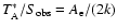 ,
where k is the
Boltzmann constant,
is the calibrated
antenna temperature outlined on Sect. 2.2 and
,
where k is the
Boltzmann constant,
is the calibrated
antenna temperature outlined on Sect. 2.2 and
 is an equivalent total flux density observed for the receiver,
Eq. (A.1) may be expressed for A100 and B100 as:
is an equivalent total flux density observed for the receiver,
Eq. (A.1) may be expressed for A100 and B100 as:
 and
and
 .
From (A.2) and (A.3) and defining
the linearly polarized flux density of the observed source
as
.
From (A.2) and (A.3) and defining
the linearly polarized flux density of the observed source
as
 ,
then it is straightforward to show
that:
,
then it is straightforward to show
that:
 can be expressed as the following function of
astronomical angles:
(t) is the electric vector
position angle of the source (defined from north to east in the equatorial
coordinate system (RA, Dec)) and
can be expressed as the following function of
astronomical angles:
(t) is the electric vector
position angle of the source (defined from north to east in the equatorial
coordinate system (RA, Dec)) and  and
and
 are,
respectively, the parallactic angle and elevation angles
(see Fig. A.1 and, Thum et al. 2000).
Note that the location of the receiver cabin in the
Nasmyth focus of the IRAM 30 m telescope causes a
rotation of the equatorial reference system by an angle
are,
respectively, the parallactic angle and elevation angles
(see Fig. A.1 and, Thum et al. 2000).
Note that the location of the receiver cabin in the
Nasmyth focus of the IRAM 30 m telescope causes a
rotation of the equatorial reference system by an angle
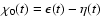 with regard to the
polarization reference system (x, y).
with regard to the
polarization reference system (x, y).
![\begin{figure}
\par\includegraphics[width=7cm,clip]{4649figa1.eps}
\end{figure}](/articles/aa/full/2006/34/aa4649-05/img266.gif) |
Figure A.1:
Angles in the reference polarization plane ( x,
y) as seen from the A100 and B100, IRAM 30 m
heterodyne receivers. ,
which is defined in
( x, y) and can be measured by fitting
Eqs. (A.5) and (A.6), relates
to the astronomical electric vector position
angle  (defined from north
to east in the equatorial coordinate system (RA, Dec), to the
parallactic angle
and to the elevation angle
.
(defined from north
to east in the equatorial coordinate system (RA, Dec), to the
parallactic angle
and to the elevation angle
. |
The statistical variables used in this paper are defined in detail by Quirrenbach et al. (2000) and Kraus et al. (2003). Here we present a summary of these definitions.
The modulation index,
 is the standard deviation of the flux
density measurements and
is the standard deviation of the flux
density measurements and
 is its average in time)
provides the strength of the observed variability amplitude
of each source without taking into account the uncertainty
of the measurements.
is its average in time)
provides the strength of the observed variability amplitude
of each source without taking into account the uncertainty
of the measurements.
The variability amplitude,
The reduced chi-squared,
 their errors) tests
the hypothesis that the measured light curves could be modelled
by a constant function. We consider that a source is variable
(with a significance level
their errors) tests
the hypothesis that the measured light curves could be modelled
by a constant function. We consider that a source is variable
(with a significance level
 %) only if its light
curve shows a probability to be constant
%) only if its light
curve shows a probability to be constant
 %.
%.
Finally, the structure function is defined as
denoting averaging in time).
A characteristic time-scale in the light curves (i.e., the time
between a maximum and a minimum or vice-versa) causes a maximum in ,
while a periodic pattern produces a minimum.
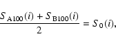
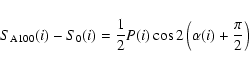
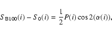
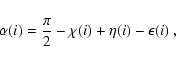
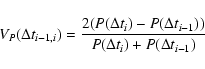
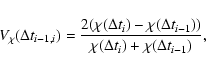
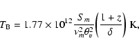
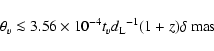
![\begin{displaymath}
\delta_{\rm {IC}} = f ( \alpha ) S_{m}
\left[ \frac {{\rm ...
... 3 \alpha ) } }
\right]^{ 1 / ( 4 - 2 \alpha ) } ( 1 + z ) ,
\end{displaymath}](/articles/aa/full/2006/34/aa4649-05/img197.gif)
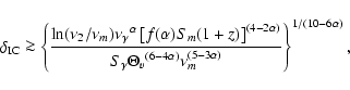
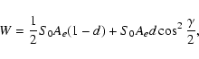


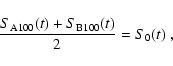
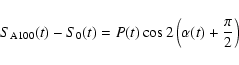
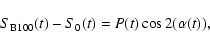
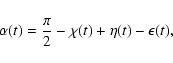
![\begin{displaymath}
m[\%]=100 \frac{\sigma_{S}}{\langle S\rangle} ,
\end{displaymath}](/articles/aa/full/2006/34/aa4649-05/img267.gif)
![\begin{displaymath}
Y[\%]=3 \sqrt{m^{2}-m_{0}^{2}} ,
\end{displaymath}](/articles/aa/full/2006/34/aa4649-05/img268.gif)