A&A 450, 777-791 (2006)
DOI: 10.1051/0004-6361:20054223
S. Bagnulo1 - J. D. Landstreet2 - E. Mason1 - V. Andretta3 - J. Silaj2 - G. A. Wade4
1 - European Southern Observatory,
Casilla 19001,
Santiago 19, Chile
2 -
Physics & Astronomy Department,
The University of Western Ontario,
London, Ontario, N6A 3K7, Canada
3 -
INAF - Osservatorio Astronomico di Capodimonte,
salita Moiariello 16, 80131 Napoli, Italy
4 -
Department of Physics,
Royal Military College of Canada,
PO Box 17000, Station "Forces''
Kingston, Ontario, K7K 7B4, Canada
Received 19 September 2005 / Accepted 12 January 2006
Abstract
Context. About 5% of upper main sequence stars are permeated by a strong magnetic field, the origin of which is still matter of debate.
Aims. With this work we provide observational material to study how magnetic fields change with the evolution of stars on the main sequence, and to constrain theory explaining the presence of magnetic fields in A and B-type stars.
Methods. Using FORS1 in spectropolarimetric mode at the ESO VLT, we have carried out a survey of magnetic fields in early-type stars belonging to open clusters and associations of various ages.
Results. We have measured the magnetic field of 235 early-type stars with a typical uncertainty of
![]() G. In our sample, 97 stars are Ap or Bp stars. For these targets, the median error bar of our field measurements was
G. In our sample, 97 stars are Ap or Bp stars. For these targets, the median error bar of our field measurements was ![]() G. A field has been detected in about 41 of these stars, 37 of which were not previously known as magnetic stars. For the 138 normal A and B-type stars, the median error bar was 136 G, and no field was detected in any of them.
G. A field has been detected in about 41 of these stars, 37 of which were not previously known as magnetic stars. For the 138 normal A and B-type stars, the median error bar was 136 G, and no field was detected in any of them.
Key words: stars: magnetic fields - stars: chemically peculiar - stars: evolution - polarization - techniques: polarimetric
Although considerable progress has been made in understanding the physical processes at work in these stars, many important problems remain unsolved. Among these are two major questions. First, although there is strong evidence (e.g., the stability of the observed fields, the lack of symptoms of Sun-like activity, and the lack of any important correlation of observed field strength with rotational angular velocity) that the observed fields are fossil fields, it is not yet clear how these fields evolve during the main sequence phase. Secondly, although it is believed that the basic mechanism leading to both chemical anomalies and to atmospheric inhomogeneities is the competition between gravitational settling, radiative levitation, and various hydrodynamic processes, the interplay of these processes is still very poorly understood.
In this situation, it is helpful to look to observations to guide physical theory. One kind of information about the magnetic Ap and Bp stars (hereafter referred to as magnetic Ap stars) that has been almost entirely lacking is the age of observed stars. Good age information would be very useful for discerning systematic evolutionary changes in field strength, chemical composition, rotation rates, etc. The general lack of useful age information about magnetic Ap stars occurs because almost all of the bright magnetic Ap stars are field stars. Even with the accurate parallaxes now available from the Hipparcos mission, the uncertainties in luminosity and effective temperature of Ap stars are large enough that placing them in the HR diagram only suffices to determine very roughly their stage of evolution (see Sect. 2.1 below).
The obvious way to obtain improved ages for magnetic Ap stars is to
observe such stars in open clusters. Until recently such a study has
not been possible because cluster Ap stars are mostly fainter than
![]() or 7, beyond the limit of accurate magnetic field
measurements with available instruments. This situation has changed
due to the development of a new generation of highly efficient
spectropolarimeters and observing strategies, and their availability
on large telescopes. In particular, the FORS1 spectropolarimeter on
one of the ESO 8 m VLT telescopes has been shown to be a powerful
tool for measuring fields in very faint Ap stars. It has recently been
used to detect a field in a star of V = 12.88, the faintest magnetic
Ap in which a field has ever been detected (Bagnulo et al.
2004).
or 7, beyond the limit of accurate magnetic field
measurements with available instruments. This situation has changed
due to the development of a new generation of highly efficient
spectropolarimeters and observing strategies, and their availability
on large telescopes. In particular, the FORS1 spectropolarimeter on
one of the ESO 8 m VLT telescopes has been shown to be a powerful
tool for measuring fields in very faint Ap stars. It has recently been
used to detect a field in a star of V = 12.88, the faintest magnetic
Ap in which a field has ever been detected (Bagnulo et al.
2004).
Another very important development has been the substantial increase in the number of probable magnetic Aps identified in clusters, particularly by the systematic surveys of Maitzen and his collaborators. Furthermore, the availability of very accurate proper motions for a very large number of stars from the Hipparcos mission and the Tycho-2 catalogue has greatly facilitated the correct separation of cluster members from foreground and background stars.
The time is now clearly ripe for studying magnetic Ap stars in
clusters to obtain for the first time a reasonably large sample of
magnetic Ap stars of known absolute and evolutionary ages. We have
started to carry out such a survey, using the FORS1
spectropolarimeter. The first stage of this survey is reported in this
paper. Section 2 discusses the rationale and scope of
this survey, in particular what the advantages are of studying open
cluster stars compared to studying field stars, why FORS1 at the VLT
is an ideal instrument for this survey, and how individual targets
have been selected. Sections 3-6 describe how the magnetic field can be
determined from observations of polarized spectra in terms of basic
physics, observing strategy, data reduction, and
![]() determination. These sections contain, for other FORS1 users, a
detailed discussion of the optimized techniques we have developed for
field measurement, and may be skipped by readers interested mainly in
the observational results. In Sects. 7 and 8 we present and discuss the observations obtained
during this survey. Conclusions are presented in
Sect. 9.
determination. These sections contain, for other FORS1 users, a
detailed discussion of the optimized techniques we have developed for
field measurement, and may be skipped by readers interested mainly in
the observational results. In Sects. 7 and 8 we present and discuss the observations obtained
during this survey. Conclusions are presented in
Sect. 9.
Temperatures for many of field stars may be estimated using available UBV, uvby, or Geneva photometry, together with calibrations provided by Stepien & Dominiczak (1989), Hauck & North (1993), and Napiwotzki et al. (1993). Luminosities require distances and bolometric corrections. Distances to many nearby Ap stars have recently been accurately determined by the Hipparcos project (see Gomez et al. 1998); for the Ap stars nearer than about 100 pc, the relative distance errors are less than about 10%. The bolometric corrections required have been discussed by Lanz (1984). Thus, it is now possible to place a large number of Ap stars on the HR diagram, and, using the evolution tracks for stars of various masses, to estimate both the mass and the age of individual stars. This exercise has been carried out by Gomez et al. (1998), by Pöhnl et al. (2005), and by Kochukhov & Bagnulo (2006) for a very large sample of nearby Ap stars, and by Hubrig et al. (2000) for a special sample of particularly slowly rotating magnetic Ap stars. In fact, as discussed below, this method is limited by large uncertainties.
Effective temperatures of magnetic Ap stars are still somewhat
uncertain, more so than for normal main sequence stars because of the
peculiar energy distributions of Ap stars (see Stepien &
Dominiczak 1989). A recent tabulation by Sokolov
(1998) of effective temperatures for nearly 70 Ap stars,
with comparisons to earlier determinations, suggests that the
uncertainty in
![]() typically about 5%, or
typically about 5%, or
![]() dex.
dex.
![\begin{figure}
\par\includegraphics[origin=rb,angle=90,width=12.4cm,clip]{4223fi...
...ncludegraphics[origin=rb,angle=90,width=12.4cm,clip]{4223fig1b.ps}
\end{figure}](/articles/aa/full/2006/17/aa4223-05/img24.gif) |
Figure 1:
Top panels: the position of a star in
the HR diagram, and the star's position transformed into a diagram of
age as a function of stellar mass, assuming that we know effective
temperature |
| Open with DEXTER | |
For Hipparcos parallaxes, the distance uncertainty at 100 pc is about 8% (or about 0.035 dex), and increases with the distance
itself. There is also an uncertainty in the appropriate bolometric
correction (BC) to apply. First of all, there is an uncertainty of
![]() mag in the estimate of the BC of a normal A-type star (due
in part to the uncertainty in
mag in the estimate of the BC of a normal A-type star (due
in part to the uncertainty in
![]() ). Then, for Ap stars, one has to
apply a correction to the normal BC. According to Lanz
(1984) this correction is uncertain by
). Then, for Ap stars, one has to
apply a correction to the normal BC. According to Lanz
(1984) this correction is uncertain by
![]() mag. Finally, there is the uncertainty as to whether one should
apply the Lutz-Kelker correction, about 0.1 mag at 100 pc. Taking
these effects together, for nearby field stars, the uncertainty in
mag. Finally, there is the uncertainty as to whether one should
apply the Lutz-Kelker correction, about 0.1 mag at 100 pc. Taking
these effects together, for nearby field stars, the uncertainty in
![]() is
is
![]() mag, i.e.,
mag, i.e.,
![]() dex in
dex in
![]() .
These uncertainties, once converted in the (
.
These uncertainties, once converted in the (![]() ,
,
![]() )
plane, correspond to age uncertainties that may be as
large as half the main sequence life.
)
plane, correspond to age uncertainties that may be as
large as half the main sequence life.
Four examples of this kind of inference are shown in the upper panel
of Fig. 1, for stars of about
![]() and
and
![]() ,
each considered for an age near the beginning of its
main sequence lifetime and near the end. Comparison is made with the
tracks of Schaller et al. (1992) for Z = 0.02. The star
positions in the HR diagram, with their uncertainties (shaded boxes), are
shown in the upper left panel. The deduced positions in the age-mass
diagram are shown in the upper right panel. It is clear that the
error boxes for observational characteristics of Ap stars translate
into ages which are sufficiently uncertain that one
cannot resolve at least the first half of the main sequence
lifetime. The situation is somewhat better near the end of the main
sequence life, where the isochrones are farther apart, but typically
an age uncertainty of the order of
,
each considered for an age near the beginning of its
main sequence lifetime and near the end. Comparison is made with the
tracks of Schaller et al. (1992) for Z = 0.02. The star
positions in the HR diagram, with their uncertainties (shaded boxes), are
shown in the upper left panel. The deduced positions in the age-mass
diagram are shown in the upper right panel. It is clear that the
error boxes for observational characteristics of Ap stars translate
into ages which are sufficiently uncertain that one
cannot resolve at least the first half of the main sequence
lifetime. The situation is somewhat better near the end of the main
sequence life, where the isochrones are farther apart, but typically
an age uncertainty of the order of ![]() % of the total main sequence
lifetime is to be expected.
% of the total main sequence
lifetime is to be expected.
A further uncertainty in the transformation from the (
![]() ,
,
![]() )
to the (
)
to the (![]() ,
,
![]() )
plane comes from the
fact that we do not know accurately the bulk chemical composition of
any field Ap star, and thus we do not know what chemical composition
should be assumed in the theoretical tracks used for the
comparison. To estimate the size of this effect, we consider the range
of abundances ([Fe/H]) present in open clusters young enough to still
have Ap stars (say
)
plane comes from the
fact that we do not know accurately the bulk chemical composition of
any field Ap star, and thus we do not know what chemical composition
should be assumed in the theoretical tracks used for the
comparison. To estimate the size of this effect, we consider the range
of abundances ([Fe/H]) present in open clusters young enough to still
have Ap stars (say
![]() ). Searching the WEBDA database
(e.g. Mermilliod & Paunzen 2003), we found that this range
is of the order of 0.4 dex. This result is confirmed by examination
of the younger clusters in the catalogue of Chen et al.
(2003). This range of abundances may represent a
reasonable estimate of the range of values of [Fe/H] present in nearby
field stars.
). Searching the WEBDA database
(e.g. Mermilliod & Paunzen 2003), we found that this range
is of the order of 0.4 dex. This result is confirmed by examination
of the younger clusters in the catalogue of Chen et al.
(2003). This range of abundances may represent a
reasonable estimate of the range of values of [Fe/H] present in nearby
field stars.
A change in [Fe/H] of 0.4 dex
corresponds to a change in metal abundance of about a factor of
2.5. This is just the difference in abundance between the evolution
calculations with Z = 0.008 and Z = 0.02 provided by the Geneva
group (Schaller et al. 1992; Schaerer et al. 1993). Repeating the transformation from the (
![]() ,
,
![]() )
to the (
)
to the (![]() ,
,
![]() )
plane for Z =
0.008, we find the results shown in the lower panels of
Fig. 1. (We have used the same values of
)
plane for Z =
0.008, we find the results shown in the lower panels of
Fig. 1. (We have used the same values of
![]() and
and
![]() as in the upper panels.) The effect of the
uncertainty in bulk chemical composition is to add roughly another
as in the upper panels.) The effect of the
uncertainty in bulk chemical composition is to add roughly another
![]() uncertainty to the deduced fraction of the main sequence
life completed by a particular star. Overall, we see that knowledge of
uncertainty to the deduced fraction of the main sequence
life completed by a particular star. Overall, we see that knowledge of
![]() and
and
![]() provides us with mass estimates accurate to
about
provides us with mass estimates accurate to
about ![]() %, but provides only poor age resolution, especially in the
first half of the main sequence life (see also Fig. 4 of
Kochukhov & Bagnulo 2006).
%, but provides only poor age resolution, especially in the
first half of the main sequence life (see also Fig. 4 of
Kochukhov & Bagnulo 2006).
The situation is substantially improved if the star is a member of a
cluster or association. The absolute age of the star is then known
with essentially the precision of the cluster age. The uncertainty of
this number varies from cluster to cluster, mainly because of the
difficulty of deciding exactly where to place the cluster turnoff.
Typically the uncertainty in
![]() is of the order of
is of the order of ![]() dex, about
dex, about ![]() % of the
absolute age (see for example Castellani et al. 1992),
although more accurate ages are sometimes reported (e.g. Carrier et al. 1999). This represents a very considerable improvement in
absolute age, especially for a star in the early part of its main
sequence life. If we know only position in the HR diagram, a star with
an actual age of 107 yr and a main sequence lifetime of 109 yr
would have an age uncertainty of the order of
% of the
absolute age (see for example Castellani et al. 1992),
although more accurate ages are sometimes reported (e.g. Carrier et al. 1999). This represents a very considerable improvement in
absolute age, especially for a star in the early part of its main
sequence life. If we know only position in the HR diagram, a star with
an actual age of 107 yr and a main sequence lifetime of 109 yr
would have an age uncertainty of the order of
![]() yr, while
the same star in a cluster would have an age uncertainty of roughly
yr, while
the same star in a cluster would have an age uncertainty of roughly
![]() yr. Only for a star in about the last third of its main
sequence life is the age uncertainty not substantially improved by
knowing that it is in a cluster. Another advantage of studying cluster
stars is that one may determine the appropriate cluster bulk
metallicity (and hence decide what evolution tracks to use for
comparison) by studying the lower main sequence stars.
yr. Only for a star in about the last third of its main
sequence life is the age uncertainty not substantially improved by
knowing that it is in a cluster. Another advantage of studying cluster
stars is that one may determine the appropriate cluster bulk
metallicity (and hence decide what evolution tracks to use for
comparison) by studying the lower main sequence stars.
The masses of cluster stars can be determined with similar methods and
similar (or better) accuracy than for local field stars. The values of
![]() are known with about the same accuracy as for local field stars,
and there are the same uncertainties for the bolometric correction.
Hipparcos parallaxes are normally not available, but the value of
luminosity is obtained from the observed V magnitude together with
the cluster's apparent distance modulus (V - MV). Recent
determinations of distance modulus by main sequence fitting appear to
achieve an accuracy of about
are known with about the same accuracy as for local field stars,
and there are the same uncertainties for the bolometric correction.
Hipparcos parallaxes are normally not available, but the value of
luminosity is obtained from the observed V magnitude together with
the cluster's apparent distance modulus (V - MV). Recent
determinations of distance modulus by main sequence fitting appear to
achieve an accuracy of about ![]() mag (e.g., Robichon et al. 1999). This accuracy is generally obtained out to
distances well beyond those few clusters for which accurate (
mag (e.g., Robichon et al. 1999). This accuracy is generally obtained out to
distances well beyond those few clusters for which accurate (![]() %)
parallaxes are available. Furthermore, if we know the cluster
metallicity, we can decide which evolution tracks to use. The
precision of the mass determination of cluster stars is about
%)
parallaxes are available. Furthermore, if we know the cluster
metallicity, we can decide which evolution tracks to use. The
precision of the mass determination of cluster stars is about ![]() % if the bulk composition is not known, and somewhat better if it
is.
% if the bulk composition is not known, and somewhat better if it
is.
Our conclusion is that an age derived using only the position in the HR diagram of an individual Ap star in the field is at present sufficiently uncertain to be of little value except for stars near the end of their main sequence lives (although important conclusions can still be drawn from statistical considerations: see Pöhnl et al. 2005 and Kochukhov & Bagnulo 2006). In contrast, if the star is a member of a cluster of known age, it is possible to determine accurately both the mass and age (or fraction of main sequence life elapsed). Therefore, the study of Ap stars that are cluster members is of great value in understanding the temporal evolution of rotation, magnetic fields, and atmospheric chemistry in all magnetic Ap stars.
At present only a few cluster Ap star candidates are known to be magnetic. The total number of clusters for which magnetic observations had been published is eight, with a total of 13 stars surveyed. In addition, extensive surveys had been carried in for the Ori OB1 (Borra 1981) and Sco OB2 associations (Thompson et al. 1987). Accordingly, we have decided to carry out a survey of magnetic stars in open clusters to provide age information for a substantial sample of Ap stars.
In principle, we may carry out a survey by searching either for
visible Zeeman splitting of spectral lines in a simple intensity
spectrum, or by searching for the circular polarization signature of a
global field of simple structure. Although Mathys and collaborators
(e.g., Mathys et al. 1997) have shown that Zeeman
splitting may be detected in some tens of field stars, this requires
quite special circumstances (i.e.,
![]() at most a few
at most a few
![]() ,
and
field strength at least 2 kG) that are not met in most of the known
magnetic Ap stars. Polarization measurement is generally a far more
sensitive and broadly-applicable method of field detection than
observation of Zeeman splitting.
,
and
field strength at least 2 kG) that are not met in most of the known
magnetic Ap stars. Polarization measurement is generally a far more
sensitive and broadly-applicable method of field detection than
observation of Zeeman splitting.
Two main methods of measurement are currently in use for detecting the
circular polarization produced by a non-zero value of
![]() .
One method
exploits the Zeeman polarization in metal lines (e.g., Babcock
1958; Preston & Stepien 1968; Mathys &
Hubrig 1997; Wade et al. 2000; Elkin et al. 2003). Field measurement by this
method usually relies on circular spectropolarimetry with a resolving
power
.
One method
exploits the Zeeman polarization in metal lines (e.g., Babcock
1958; Preston & Stepien 1968; Mathys &
Hubrig 1997; Wade et al. 2000; Elkin et al. 2003). Field measurement by this
method usually relies on circular spectropolarimetry with a resolving
power
![]() .
If the star is quite bright, with a
.
If the star is quite bright, with a
![]() value smaller than, say, 15 or 20
value smaller than, say, 15 or 20
![]() and a rich spectrum, field
errors
and a rich spectrum, field
errors ![]() as small as a few G can be achieved (Shorlin et al. 2002). On the other hand, the measurement uncertainty
depends strongly on spectral type (which determines the number of
usable lines and their intrinsic depths) and on
as small as a few G can be achieved (Shorlin et al. 2002). On the other hand, the measurement uncertainty
depends strongly on spectral type (which determines the number of
usable lines and their intrinsic depths) and on
![]() .
In
observations collecting similar total numbers of photons, the standard
error of field measurement can vary by a factor of order 102.
.
In
observations collecting similar total numbers of photons, the standard
error of field measurement can vary by a factor of order 102.
A second method employs the Zeeman polarization in
the wings of the Balmer lines. These lines may be
observed with quite low resolving power (
![]() ), using either
interference filters (e.g., Borra & Landstreet 1980) or a
low-dispersion spectrograph (Bagnulo et al. 2002). Since
the Balmer lines are intrinsically broad, the polarization
signal may be a factor of 10 smaller than in the metal lines, and the
best achievable standard errors are of order 30-50 G (Landstreet
1982). However, since the Balmer lines are always quite deep,
and do not vary much in strength among A and B stars, and since the
overall profile at
), using either
interference filters (e.g., Borra & Landstreet 1980) or a
low-dispersion spectrograph (Bagnulo et al. 2002). Since
the Balmer lines are intrinsically broad, the polarization
signal may be a factor of 10 smaller than in the metal lines, and the
best achievable standard errors are of order 30-50 G (Landstreet
1982). However, since the Balmer lines are always quite deep,
and do not vary much in strength among A and B stars, and since the
overall profile at
![]() is hardly affected by rotation,
this method can provide standard errors that are fairly uniform simply
by surveying a sample of stars to a specified signal-to-noise ratio.
is hardly affected by rotation,
this method can provide standard errors that are fairly uniform simply
by surveying a sample of stars to a specified signal-to-noise ratio.
The (spectro-)polarimeters now in use make both kinds of field
measurement. However, limitations imposed by low overall efficiency
and (usually) modest telescope aperture have limited most of the
![]() field measurements to stars not much fainter than V = 6. This
magnitude limit has effectively prevented any serious survey of
magnetic fields in cluster Ap stars, as only a handful of clusters and
associations have a significant number of Ap stars brighter than V =
6. With a limiting magnetic around V = 6, one is restricted to
clusters and associations not much more than 100 pc away, since the
absolute magnitude of an Ap star is typically in the range of
field measurements to stars not much fainter than V = 6. This
magnitude limit has effectively prevented any serious survey of
magnetic fields in cluster Ap stars, as only a handful of clusters and
associations have a significant number of Ap stars brighter than V =
6. With a limiting magnetic around V = 6, one is restricted to
clusters and associations not much more than 100 pc away, since the
absolute magnitude of an Ap star is typically in the range of
![]() to +1. Only half a dozen clusters are this near.
to +1. Only half a dozen clusters are this near.
The development of the FORS1 spectropolarimeter for the ESO Very Large
Telescope (VLT) has changed the situation dramatically. FORS1
incorporates a multi-object low dispersion spectrograph with
polarizing optics. In polarimetric mode, spectra with
![]() may be obtained for up to nine objects simultaneously in a field 7'square. Bagnulo et al. (2002) have shown that FORS1 can
be used very effectively as a Balmer-line polarimeter for field
measurement. Since this instrument is mounted on an 8 m telescope,
and has a very high throughput, the limiting magnitude is much fainter
than with earlier instruments. Bagnulo et al. (2004) have
used FORS1 to detect a field in a star of
may be obtained for up to nine objects simultaneously in a field 7'square. Bagnulo et al. (2002) have shown that FORS1 can
be used very effectively as a Balmer-line polarimeter for field
measurement. Since this instrument is mounted on an 8 m telescope,
and has a very high throughput, the limiting magnitude is much fainter
than with earlier instruments. Bagnulo et al. (2004) have
used FORS1 to detect a field in a star of
![]() in 2.8 h
of observation, and showed that it is possible to reach a precision of
in 2.8 h
of observation, and showed that it is possible to reach a precision of
![]() G in about 1 h of integration at V =
10. With a limiting magnitude of 10 or even fainter, we can survey
clusters and associations out to several hundred pc, and the number of
clusters that can be studied rises to roughly 100. In addition
Bagnulo et al. (2002) have shown that the low resolution
does not prevent the use of metal lines to measure the magnetic field
in stars with rich metallic spectra. This fact may be used to increase
the sensitivity of field measurements in some stars. A third advantage
of FORS1 is that in clusters, it is often possible to observe several
stars simultaneously. We have used this capability to observe multiple
Ap candidate stars, but also non-Ap cluster members in the hopes of
making serendipitous field detections.
G in about 1 h of integration at V =
10. With a limiting magnitude of 10 or even fainter, we can survey
clusters and associations out to several hundred pc, and the number of
clusters that can be studied rises to roughly 100. In addition
Bagnulo et al. (2002) have shown that the low resolution
does not prevent the use of metal lines to measure the magnetic field
in stars with rich metallic spectra. This fact may be used to increase
the sensitivity of field measurements in some stars. A third advantage
of FORS1 is that in clusters, it is often possible to observe several
stars simultaneously. We have used this capability to observe multiple
Ap candidate stars, but also non-Ap cluster members in the hopes of
making serendipitous field detections.
This survey is biased toward stars with longitudinal field of absolute
value larger than about 200-300 G, but is not biased with respect
to ![]() .
Any bias with respect to spectral type is primarily a
feature of the previous classification programmes that have identified
candidate magnetic Ap stars in clusters, rather than a feature imposed by
an instrumental field detection sensitivity that depends on the star's
spectroscopic features.
.
Any bias with respect to spectral type is primarily a
feature of the previous classification programmes that have identified
candidate magnetic Ap stars in clusters, rather than a feature imposed by
an instrumental field detection sensitivity that depends on the star's
spectroscopic features.
Numerous studies have identified probable Ap members of clusters and
associations. Surveys for Ap/Bp cluster members based on
low-dispersion spectroscopy were reported by Hartoog (1976,
1977), and by Abt (1979). Probable Ap stars have also
been reported from a number of studies of individual clusters
(e.g. Dachs & Kabus 1989). Furthermore, the Michigan
Spectral Survey (e.g. Houk & Smith-Moore 1988) has
provided uniform MK classifications for a large number of HD stars in
the fields of clusters south of
![]() .
This allowed us
to select some Ap stars that are possible cluster members.
.
This allowed us
to select some Ap stars that are possible cluster members.
Another important source of identifications of cluster Ap stars has
been the use of photometric indices that are sensitive to a broad
depression near 5200 Å in the energy distribution of most Ap stars
(e.g., Kupka et al. 2003). In particular,
Maitzen and collaborators (e.g., Maitzen 1993) have developed
a narrow band photometric index (![]() )
which is reasonably
sensitive to the spectral peculiarities of Ap stars with effective
temperatures in the range
)
which is reasonably
sensitive to the spectral peculiarities of Ap stars with effective
temperatures in the range
![]() K. Maitzen's group
has systematically obtained
K. Maitzen's group
has systematically obtained ![]() photometry of many clusters
to identify Ap stars. The
photometry of many clusters
to identify Ap stars. The ![]() system has also been used
by Joncas & Borra (1981) to search for Ap stars in the
Orion OB1 association.
system has also been used
by Joncas & Borra (1981) to search for Ap stars in the
Orion OB1 association.
It is also known that the Z index, which can be
computed for the many cluster stars for which Geneva photometry is
available, is a powerful discriminant of Ap stars in
approximately the same temperature range as the ![]() index
(e.g. Kramer & Maeder 1980; Hauck & North
1982).
index
(e.g. Kramer & Maeder 1980; Hauck & North
1982).
We have made extensive use of the WEBDA cluster database (e.g. Mermilliod & Paunzen 2003), Simbad, and a catalogue of candidate cluster Ap stars by Renson (1992).
Most of the surveys discussed above have made a serious effort to determine cluster memberships, mainly on the basis of spatial location and apparent magnitude. However, recent work based on and stimulated by the Hipparcos astrometric space mission has led to a major expansion in the available data on parallaxes and proper motions. Hipparcos parallaxes (e.g. Gomez et al. 1998) provide a valuable membership discriminant out to about 300 pc for many cluster stars. Even more importantly, the Tycho (Høg et al. 1998) and Tycho-2 (Høg et al. 2000) proper motion catalogues now provide powerful tests of membership out to nearly one kpc, for a much larger number of stars, as demonstrated for example by Robichon et al. (1999), de Zeeuw et al. (1999), and Dias et al. (2001).
Using the resources discussed above, a database containing a variety of information on more than 200 suspected Ap cluster members in more than 70 clusters and associations was constructed and used for the selection of the targets. In general, we have given highest priority to stars which appear to be probable Ap stars, and probable cluster members, but we have also observed a number of stars for which at least one of these criteria was uncertain. Up to the present time, we have been able to observe (or occasionally find in the literature) magnetic observations of about 1/3 of the stars in our database.
Cluster membership will be discussed in the second paper in this series (Landstreet et al., in preparation, hereafter referred to as Paper II), where we will analyze the astrophysical and evolutionary results of our survey in more detail. The present paper focuses on the magnetic observations themselves.
The mean longitudinal magnetic field
![]() ,
i.e., the
component of the magnetic field along the line of sight averaged over
the visible stellar disk, can be measured through the analysis of the
circular polarization of spectral lines. In the weak
field regime (i.e., when the Zeeman splitting is small compared to
the line intrinsic broadening) we have (e.g. Landstreet 1982)
,
i.e., the
component of the magnetic field along the line of sight averaged over
the visible stellar disk, can be measured through the analysis of the
circular polarization of spectral lines. In the weak
field regime (i.e., when the Zeeman splitting is small compared to
the line intrinsic broadening) we have (e.g. Landstreet 1982)
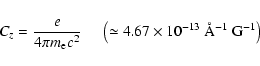 |
(2) |
A least-squares technique can be used to derive the longitudinal field
via Eq. (1). We minimise the expression
The application of a least-squares technique is justified if
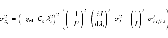 |
(6) |
![\begin{displaymath}\sigma^2_{y_i} = \sigma^2\left[(V/I)_i\right].
\end{displaymath}](/articles/aa/full/2006/17/aa4223-05/img70.gif)
For this study, grism 600 B seems a better choice than 600 R.
Although H![]() is more sensitive to the magnetic field
than individual H Balmer lines at shorter wavelengths (the Zeeman
effect depends quadratically upon wavelength), the combined analysis
of several Balmer lines from H
is more sensitive to the magnetic field
than individual H Balmer lines at shorter wavelengths (the Zeeman
effect depends quadratically upon wavelength), the combined analysis
of several Balmer lines from H![]() down to the Balmer jump leads to
a smaller error bar than the analysis of H
down to the Balmer jump leads to
a smaller error bar than the analysis of H![]() only. Furthermore,
the flux of an A-type stars is larger in the blue than in the red,
therefore the same SNR can be reached with a shorter integration time
using grism 600 B rather than grism 600 R. On the other hand, it
should be noted that the useful field of view in fims mode
depends on the spectral range that one wishes to cover: the larger the
spectral range that one needs to observe, the smaller the spatial
region where one can place slitlets. Hence, in fims mode,
grism 600 R offers more flexibility than grism 600 B, as its useful
wavelength coverage corresponds to H
only. Furthermore,
the flux of an A-type stars is larger in the blue than in the red,
therefore the same SNR can be reached with a shorter integration time
using grism 600 B rather than grism 600 R. On the other hand, it
should be noted that the useful field of view in fims mode
depends on the spectral range that one wishes to cover: the larger the
spectral range that one needs to observe, the smaller the spatial
region where one can place slitlets. Hence, in fims mode,
grism 600 R offers more flexibility than grism 600 B, as its useful
wavelength coverage corresponds to H![]() only, which does not put
a strong constraint on the field of view. In (ESO period)
P68 we used grism 600 R (in combination with the order
separation filter GG 435). In P70, P72, P73, and P74, we
used grism 600 B (with no order separation filter).
only, which does not put
a strong constraint on the field of view. In (ESO period)
P68 we used grism 600 R (in combination with the order
separation filter GG 435). In P70, P72, P73, and P74, we
used grism 600 B (with no order separation filter).
For most of the observations, we have used a slit width of 0.5
![]() or 0.8
or 0.8
![]() .
.
The data have been reduced and optimally extracted using standard IRAF routines. All the science frames have been bias subtracted with the corresponding master bias obtained from a series of five frames taken the morning after the observations. No flat fielding procedure has been applied to our data. By performing reduction experiments with and without flat-fielding, we have verified that flat fielding does not influence significantly the final computation of the Stokes profiles. In fact, flat fields obtained with the grism 600 B are severely affected by internal reflections from the Longitudinal Atmospheric Dispersion Corrector (LADC). Frames obtained in fims mode were read out in four ports. The CCD is thus divided in four quadrants, each of them characterized by its own bias level and gain. In order to compensate for the different gains, we multiplied each science frames by the ratio of an imaging screen flat read out in one port and an imaging screen flat read out in four ports.
When extracting the spectra we found that the use of standard
extraction apertures (![]() pixels width) introduced artefacts
into the Stokes V spectrum. This problem was solved using
apertures as large as
pixels width) introduced artefacts
into the Stokes V spectrum. This problem was solved using
apertures as large as
![]() times the spatial FWHM of the
spectrum, i.e., typically 50 pixels width. Apertures that are not symmetric
about the flux peak have been used for stars close to the edge of the
slit. This occurred occasionally for targets observed in fims
mode. We used a high-order (
times the spatial FWHM of the
spectrum, i.e., typically 50 pixels width. Apertures that are not symmetric
about the flux peak have been used for stars close to the edge of the
slit. This occurred occasionally for targets observed in fims
mode. We used a high-order (![]() )
Legendre fitting function to
trace the spectrum
)
Legendre fitting function to
trace the spectrum![]() . Lower order functions were
used only in the case of low SNR secondary targets (typically in
frames obtained in fims mode) and/or in the case of spectra
the length of which occupied just a fraction of the CCD (again in
fims frames, depending on the positioning of the slitlets).
. Lower order functions were
used only in the case of low SNR secondary targets (typically in
frames obtained in fims mode) and/or in the case of spectra
the length of which occupied just a fraction of the CCD (again in
fims frames, depending on the positioning of the slitlets).
Sky subtraction was performed differently for spectra obtained in fast and fims mode. In the first case the sky subtraction was performed selecting symmetric regions on the left and right side of each spectrum (typically between pixel 40 and 50 from the central peak), and fitting those with a Chebyshev polynomial. In the case of data obtained in fims mode, whenever the star was not positioned at the center of the slitlet, the sky was estimated on just one region at one side of the spectrum. In fact, we found that sky-subtraction is not critical in the sense that it does not significantly affect the final results. In some cases, we preferred not to perform sky-subtraction at all, because of the presence of LADC reflections close to the spectrum.
The FORS1 calibration plan includes wavelength calibrations frames obtained at all retarder waveplate positions used for the science. However, we found that the best and safest strategy is to use, for a complete set of science data, just a single wavelength calibration frame, and not match science and wavelength calibration frames according to their retarder waveplate angles. We found that this latter method occasionally introduces spurious polarization signals.
Wavelength calibration typically led to RMS scatter of
![]() pixels and maximum error of
pixels and maximum error of ![]() km s-1. The fine
tuning of wavelength calibration based on night sky lines could not be
performed. Therefore the accuracy of the wavelength calibration is
restricted by instrument flexures, which are expected to be less than
1 pixel up to a zenith distance of 60
km s-1. The fine
tuning of wavelength calibration based on night sky lines could not be
performed. Therefore the accuracy of the wavelength calibration is
restricted by instrument flexures, which are expected to be less than
1 pixel up to a zenith distance of 60![]() (see FORS1/2 User Manual).
Numerical tests show that this is of negligible impact on the
determination of the mean longitudinal magnetic field, using the
method described by Bagnulo et al. (2002) and elaborated
below.
(see FORS1/2 User Manual).
Numerical tests show that this is of negligible impact on the
determination of the mean longitudinal magnetic field, using the
method described by Bagnulo et al. (2002) and elaborated
below.
The error bar associated with the Stokes V/I, computed via
Eq. (7) is
In order to detect weak magnetic fields (![]() G) with the
technique used in this work, one has to obtain ultra high SNR (
G) with the
technique used in this work, one has to obtain ultra high SNR (
![]() Å-1) observations. Even with a 8 m telescope, this can be
achieved only on relatively bright stars (
Å-1) observations. Even with a 8 m telescope, this can be
achieved only on relatively bright stars (![]() ,
if we limit the
shutter time to
,
if we limit the
shutter time to ![]() h). Due to the limited CCD well capacity, multiple
exposures have to be taken. From a practical point of view, one has
to set the exposure time to a value that maximises the photon count
without risk of CCD saturation (e.g., by adjusting the exposure time to
get a peak count of 30 000 ADU per pixel), and then take several
pairs of exposures with the retarder waveplate at the
h). Due to the limited CCD well capacity, multiple
exposures have to be taken. From a practical point of view, one has
to set the exposure time to a value that maximises the photon count
without risk of CCD saturation (e.g., by adjusting the exposure time to
get a peak count of 30 000 ADU per pixel), and then take several
pairs of exposures with the retarder waveplate at the
![]() and
and
![]() positions. Equation (10) can be explicitly
expressed in terms of ADU in the following way. Let us define
M as the ADU per pixel and g as the number of electrons per
ADU, so that actual photon count
positions. Equation (10) can be explicitly
expressed in terms of ADU in the following way. Let us define
M as the ADU per pixel and g as the number of electrons per
ADU, so that actual photon count
![]() is given by gM. Let
us also define
is given by gM. Let
us also define
![]() as the ratio between the ADU
integrated in a pixel column along the direction perpendicular to the
dispersion, and the peak ADU in the central
pixel. The error bar on the circular polarization measured in the
wavelength interval
as the ratio between the ADU
integrated in a pixel column along the direction perpendicular to the
dispersion, and the peak ADU in the central
pixel. The error bar on the circular polarization measured in the
wavelength interval
![]() covered by 1 pixel is given by
covered by 1 pixel is given by
 =
\frac{1}{4~m~g~\mathcal{A}_{\rm s}~M_{\rm max}}
\end{displaymath}](/articles/aa/full/2006/17/aa4223-05/img99.gif)
Recalling the properties of a Gaussian, we can write
![]() FWHM. With a plate scale of 0.2
FWHM. With a plate scale of 0.2
![]() per pixel, as in the case of FORS1, and with 0.8
per pixel, as in the case of FORS1, and with 0.8
![]() seeing,
seeing,
![]() .
Assuming g=2.9 (a
typical value for the FORS1 "low gain'' readout mode), and setting as
a peak value
.
Assuming g=2.9 (a
typical value for the FORS1 "low gain'' readout mode), and setting as
a peak value
![]() ADU, we get
ADU, we get
We found that measuring V/I with an accuracy of a few units in
10-4 per Å in the continuum near to H![]() allowed us to
measure magnetic fields with an error bar between 50 and
100 G. Therefore, we decided that our observing strategy would be
based on a series of four pairs of exposures (following the sequence
allowed us to
measure magnetic fields with an error bar between 50 and
100 G. Therefore, we decided that our observing strategy would be
based on a series of four pairs of exposures (following the sequence
![]() ,
,
![]() ,
,
![]() ,
,
![]() ,
etc.). However, we could limit the number of pairs of exposure to four
only when we obtained telescope time in visitor mode, which allowed us
to optimize the exposure time based on the weather conditions. During P72 and P73 we were allocated telescope time in service
mode, and were forced to set the exposure time to
conservatively low values to be sure to avoid CCD saturation. In
these cases the number of pairs of exposures was increased from four
to six or eight to guarantee a sufficient SNR.
,
etc.). However, we could limit the number of pairs of exposure to four
only when we obtained telescope time in visitor mode, which allowed us
to optimize the exposure time based on the weather conditions. During P72 and P73 we were allocated telescope time in service
mode, and were forced to set the exposure time to
conservatively low values to be sure to avoid CCD saturation. In
these cases the number of pairs of exposures was increased from four
to six or eight to guarantee a sufficient SNR.
Thought must be given to the ratio between shutter time and overhead
time, as the latter (![]() min for a series of 4 pairs of
exposures) may represent a substantial fraction of the total
time for a single pointing.
Using grism 600 B with a 0.5
min for a series of 4 pairs of
exposures) may represent a substantial fraction of the total
time for a single pointing.
Using grism 600 B with a 0.5
![]() slit width, we can obtain
a peak ADU count of
slit width, we can obtain
a peak ADU count of
![]() in about 10 min shutter time
for a V=11-12 A-type star (depending on the weather conditions), and
in just 1 min for
V=8.5-9.5.
in about 10 min shutter time
for a V=11-12 A-type star (depending on the weather conditions), and
in just 1 min for
V=8.5-9.5.
Table 1:
![]() measurements of the V=6.1 Ap star
HD 94660 = KQ Vel. Date, UT, and signal to noise ratio (SNR) are
calculated as explained in the caption of Table A.3. Observations
obtained in P66 had been already published by Bagnulo et al. (2002).
measurements of the V=6.1 Ap star
HD 94660 = KQ Vel. Date, UT, and signal to noise ratio (SNR) are
calculated as explained in the caption of Table A.3. Observations
obtained in P66 had been already published by Bagnulo et al. (2002).
If no value in the m2 set of
(V/I)ij pairs has been rejected, and
if we assume that the errors given by Eq. (9) are approximately
equal for all spectra, we can estimate the error bar of
![]() as:
as:
We encountered a number of cases for which the field was detected at
about 3-![]() level, and where minor changes in the data reduction
would transform a marginal detection in a null or in a definite
detection. Although these cases should certainly be investigated via
additional observations, we tried to extract further information from
the available spectra, to formulate a more robust and
reliable criterion for field detection.
level, and where minor changes in the data reduction
would transform a marginal detection in a null or in a definite
detection. Although these cases should certainly be investigated via
additional observations, we tried to extract further information from
the available spectra, to formulate a more robust and
reliable criterion for field detection.
First, we decided to explore an alternative method for the
determination of the mean longitudinal field. From the individual
pairs of
Vij/Iij and Iij given by
Eqs. (12), we calculated m2
![]() values, and
the weighted mean longitudinal field
values, and
the weighted mean longitudinal field
![\begin{displaymath}\sigma^2\left[\ensuremath{\langle B_z\rangle} '\right] = \fra...
...{ij} - \ensuremath{\langle B_z\rangle} ')^2}{m^2 (m - 1)}\cdot
\end{displaymath}](/articles/aa/full/2006/17/aa4223-05/img126.gif)
Second, we performed a systematic analysis of metal lines. As pointed
out earlier, Eq. (1) is formally valid only under the
weak-field approximation. Therefore, in principle,
![]() measurements
by our method should be performed only on H Balmer lines. Furthermore,
H Balmer lines are well sampled even at the low resolution of our
observations, whereas metal lines are unresolved. Nevertheless, we
found that the
measurements
by our method should be performed only on H Balmer lines. Furthermore,
H Balmer lines are well sampled even at the low resolution of our
observations, whereas metal lines are unresolved. Nevertheless, we
found that the
![]() determined via metal line analysis is consistent
with that measured from H Balmer lines, provided that
determined via metal line analysis is consistent
with that measured from H Balmer lines, provided that
![]() is
is ![]() G (see Sect. 6.2). Therefore we decided to analyze
the metal lines, i.e., to apply the least-squares
technique to spectral regions free from H Balmer lines. In
addition, we determined
G (see Sect. 6.2). Therefore we decided to analyze
the metal lines, i.e., to apply the least-squares
technique to spectral regions free from H Balmer lines. In
addition, we determined
![]() using the whole spectrum, i.e., including
both Balmer and metal lines. The outcome of this analysis will be
discussed in Sect. 6.
using the whole spectrum, i.e., including
both Balmer and metal lines. The outcome of this analysis will be
discussed in Sect. 6.
In order to compare our results with those obtained through different
techniques, we repeatedly observed a well known magnetic Ap
star: HD 94660 (=KQ Vel). Previous
![]() measurements of HD 94660 were
obtained using the H
measurements of HD 94660 were
obtained using the H![]() Balmer line (Borra & Landstreet
1975), the H
Balmer line (Borra & Landstreet
1975), the H![]() Balmer line (Bohlender et al. 1993), and metallic lines (Mathys 1994; Mathys
& Hubrig 1997). Moreover, HD 94660 is the star observed
by Bagnulo et al. (2002) to develop the technique used in
this work.
Balmer line (Bohlender et al. 1993), and metallic lines (Mathys 1994; Mathys
& Hubrig 1997). Moreover, HD 94660 is the star observed
by Bagnulo et al. (2002) to develop the technique used in
this work.
The log of our observations and
![]() measurements is given in
Table 1. Note that on 2002-02-04 we obtained two
consecutive
measurements is given in
Table 1. Note that on 2002-02-04 we obtained two
consecutive
![]() measurements: the first one with grism 600 B, the
second one with grism 600 R.
measurements: the first one with grism 600 B, the
second one with grism 600 R.
Figure 2 shows the
![]() measurements obtained from both
the Balmer and the metal lines. The
measurements obtained from both
the Balmer and the metal lines. The
![]() values obtained from the
Balmer lines blueward of H
values obtained from the
Balmer lines blueward of H![]() are consistent among themselves, and
marginally consistent with the
are consistent among themselves, and
marginally consistent with the
![]() value obtained from
H
value obtained from
H![]() .
With the exception of the measurement taken on 2001-03-22,
the
.
With the exception of the measurement taken on 2001-03-22,
the
![]() values obtained from the metal lines are not consistent with
those obtained from Balmer lines. This is probably due to the fact
that Eq. (1) is valid only under the weak field approximation
(which in this case is correct for Balmer lines but not for metal
lines). Note also that the
values obtained from the metal lines are not consistent with
those obtained from Balmer lines. This is probably due to the fact
that Eq. (1) is valid only under the weak field approximation
(which in this case is correct for Balmer lines but not for metal
lines). Note also that the
![]() values measured via metal line
analysis are not consistent among themselves if we compare data
obtained with grism 600 B and grism 600 R. The comparison between
values measured via metal line
analysis are not consistent among themselves if we compare data
obtained with grism 600 B and grism 600 R. The comparison between
![]() values obtained from H Balmer lines and metal lines will be
further discussed in Sect. 6.2.
values obtained from H Balmer lines and metal lines will be
further discussed in Sect. 6.2.
We also compared our
![]() determinations of Table 1
with those previously obtained in the literature, adopting for the
star's rotation period 2800 d (Landstreet & Mathys 2000).
The results are shown in Fig. 3. In general, it appears
that
determinations of Table 1
with those previously obtained in the literature, adopting for the
star's rotation period 2800 d (Landstreet & Mathys 2000).
The results are shown in Fig. 3. In general, it appears
that
![]() values obtained from Balmer lines are not
consistent with the
values obtained from Balmer lines are not
consistent with the
![]() determinations obtained using metallic lines.
It seems likely that different methods used to evaluate
determinations obtained using metallic lines.
It seems likely that different methods used to evaluate
![]() bear
systematic differences (even though each may be internally
consistent). Systematic inconsistencies between
bear
systematic differences (even though each may be internally
consistent). Systematic inconsistencies between
![]() determinations
in Ap stars obtained with different chemical elements or with
different techniques have been already found in previous works (see,
for instance, Ryabchikova et al. 2005, who analysed several observations of HD 24712).
determinations
in Ap stars obtained with different chemical elements or with
different techniques have been already found in previous works (see,
for instance, Ryabchikova et al. 2005, who analysed several observations of HD 24712).
![\begin{figure}
\par\includegraphics[width=8.8cm,clip]{4223fig2.ps}
\end{figure}](/articles/aa/full/2006/17/aa4223-05/img130.gif) |
Figure 2:
|
| Open with DEXTER | |
![\begin{figure}
\par\includegraphics[width=8.8cm,clip]{4223fig3.ps}
\end{figure}](/articles/aa/full/2006/17/aa4223-05/img131.gif) |
Figure 3:
Longitudinal field determinations of
HD 94660. The solid line is a fit to the
|
| Open with DEXTER | |
Figure 4 shows the
![]() values obtained from metal
lines versus those obtained from Balmer lines for the observed Ap
stars. It appears that the two methods give consistent
values obtained from metal
lines versus those obtained from Balmer lines for the observed Ap
stars. It appears that the two methods give consistent
![]() values for
values for
![]() G. Above the 1 kG level, differences
between Balmer line and metal line technique become noticeable or even
striking. E.g., for HD 310187 we obtained from the Balmer lines
G. Above the 1 kG level, differences
between Balmer line and metal line technique become noticeable or even
striking. E.g., for HD 310187 we obtained from the Balmer lines
![]() G, and from the metal lines we obtained
G, and from the metal lines we obtained
![]() G. In general, above the 1 kG level, the modulus of
G. In general, above the 1 kG level, the modulus of
![]() determined from Balmer lines is larger than that from the metal lines,
as we would expect from the earlier breakdown of the weak field
expression for metal lines.
determined from Balmer lines is larger than that from the metal lines,
as we would expect from the earlier breakdown of the weak field
expression for metal lines.
![\begin{figure}
\par\includegraphics[width=8.8cm,clip]{4223fig4.ps}
\end{figure}](/articles/aa/full/2006/17/aa4223-05/img136.gif) |
Figure 4:
|
| Open with DEXTER | |
![\begin{figure}
\par\includegraphics[angle=90,width=8.5cm,clip]{4223fig5.ps}
\end{figure}](/articles/aa/full/2006/17/aa4223-05/img137.gif) |
Figure 5:
Histograms of the error bars for the
|
| Open with DEXTER | |
Summarizing, it appears that if the field is weak, both methods are consistent, and each gives an indication whether the star is magnetic or not independent of the other.
Figure 5 compares the distributions of the error
bars for
![]() obtained via Balmer and metal line analysis for the
observed Ap stars. We see that the distribution of the error bars
calculated via metal line analysis is broader than that obtained from
Balmer lines. This is due primarily to the fact that Balmer lines have
similar strength in all A and B-type stars, whereas metal lines may
change greatly from star to star. For a given SNR, the error
bars obtained via metal line analysis are smaller in spectra that are
richer in metal lines than in spectra that are poorer in metal
lines. As expected, for a set of observations of similar SNR, the
Balmer line analysis leads to results characterised by more
homogeneous error bars than the metal line analysis.
obtained via Balmer and metal line analysis for the
observed Ap stars. We see that the distribution of the error bars
calculated via metal line analysis is broader than that obtained from
Balmer lines. This is due primarily to the fact that Balmer lines have
similar strength in all A and B-type stars, whereas metal lines may
change greatly from star to star. For a given SNR, the error
bars obtained via metal line analysis are smaller in spectra that are
richer in metal lines than in spectra that are poorer in metal
lines. As expected, for a set of observations of similar SNR, the
Balmer line analysis leads to results characterised by more
homogeneous error bars than the metal line analysis.
Table 2:
List of open clusters observed in this
survey, with approximate ages (Col. 4) and distance moduli
![]() (Col. 5) extracted from WEBDA. Column 6 gives the number of
candidate peculiar stars and Col. 7 the number of non chemically
peculiar A and B stars that we observed in each cluster.
(Col. 5) extracted from WEBDA. Column 6 gives the number of
candidate peculiar stars and Col. 7 the number of non chemically
peculiar A and B stars that we observed in each cluster.
In this survey we have observed 97 Ap stars, 138 normal A and B-type
stars, and 22 non early-type stars. All these stars are candidate
members of the open clusters (or the associations) listed in
Table 2. Figure 6 gives an
overview of the range in age and distance modulus of the target
clusters, compared to all Milky Way open clusters with known age
and
![]() .
A summary of the observing log is given
in Table 3.
.
A summary of the observing log is given
in Table 3.
Target Ap stars have been selected as explained in Sect. 2.3, and are listed in Table A.1, together with the V magnitude and the spectral type extracted from the General Catalogue of Ap and Am stars (Renson et al. 1992), and from SIMBAD. Searching the literature (in particular the catalogue by Bychkov et al. 2003), we found that 10 of these Ap stars have already been checked for magnetic field in previous studies. We observed some of our objects more than once (we have made 121 observations of Ap stars). In total we obtained 52 field detections in 41 different stars (although for five stars we have only marginal detections). Thirty-seven Ap stars in which we have detected a field were not previously known as magnetic. A few Ap stars of Table A.1 are in fact cluster non-members. Chemical peculiarity, and, above all, cluster membership, will be further discussed in Paper II, where we will also provide estimates for star's temperature, mass, and evolutionary state. Two remarkable stars have been the subject of previous papers: HD 66318 (Bagnulo et al. 2003) and NGC 2244 338 (Bagnulo et al. 2004).
The normal A and B-type stars observed in this survey are listed in
Table A.2, together with their V magnitudes and
spectral classifications. In many cases the spectral type was not
available in SIMBAD or in the literature, therefore, it has been
determined through their color indices B-V and U-B extracted from
WEBDA. The observed color indices have been corrected for extinction
using the cluster E(B-V) (also reported in WEBDA) and
applying the extinction law by Cardelli et al.
(1983). The dereddened colours have been then compared to
those of typical main sequence stars to determine the approximate
spectral type of each object. FORS1 spectra were used to roughly check
the validity of this spectral classification, but no attempt was made
to refine it. The spectral type obtained from the colour indices are
reported between squared brackets, and should be used with caution. We
discovered a posteriori that the spectra of ![]() normal
stars were in fact not of early-type. These cases are listed in
Table A.5. We do not report observations of a few
additional targets which have spectra with a too low SNR to be useful
for magnetic studies.
normal
stars were in fact not of early-type. These cases are listed in
Table A.5. We do not report observations of a few
additional targets which have spectra with a too low SNR to be useful
for magnetic studies.
Table 3: Log of the various observing runs with FORS1 at the ESO VLT, dedicated to the open cluster survey.
![\begin{figure}
\par\includegraphics[width=8.4cm,clip]{4223fig6.ps}
\end{figure}](/articles/aa/full/2006/17/aa4223-05/img140.gif) |
Figure 6:
Distance modulus versus age of open
clusters. The empty circles show all open clusters with known age
and
|
| Open with DEXTER | |
In this work we report the
![]() values obtained from the analysis of
both Balmer lines and metal lines. For peculiar stars, the medians of
the errors obtained from the Balmer lines and from the metal lines are
78 G, and 130 G, respectively. For normal stars they are 136 G, and
173 G, respectively. For normal stars the median error bar is larger
than for peculiar stars because we optimized integration times to
reach the highest possible SNR for Ap stars, rather than for the
secondary targets added in the fims mode observations. In
addition, we calculated the field measured from the analysis of the
whole spectrum, including metal lines.
The latter method formally gives
values obtained from the analysis of
both Balmer lines and metal lines. For peculiar stars, the medians of
the errors obtained from the Balmer lines and from the metal lines are
78 G, and 130 G, respectively. For normal stars they are 136 G, and
173 G, respectively. For normal stars the median error bar is larger
than for peculiar stars because we optimized integration times to
reach the highest possible SNR for Ap stars, rather than for the
secondary targets added in the fims mode observations. In
addition, we calculated the field measured from the analysis of the
whole spectrum, including metal lines.
The latter method formally gives
![]() values with the
smallest error bar: for Ap stars the median is 62 G, and for
normal stars is 94 G. Although some caution is required in
interpreting a
values with the
smallest error bar: for Ap stars the median is 62 G, and for
normal stars is 94 G. Although some caution is required in
interpreting a
![]() determination obtained combining Balmer and metal
lines, one can reasonably argue that this method may be used to
reinforce the conclusions achieved with the two primary methods.
determination obtained combining Balmer and metal
lines, one can reasonably argue that this method may be used to
reinforce the conclusions achieved with the two primary methods.
The
![]() determinations for Ap stars and for normal A and B stars are
reported in Tables A.3 and A.4,
respectively. These tables are organized as follows. The day and time
of the observations are given in Cols. 2, and 3, respectively, and
correspond to the midpoint between the instant when the shutter opens
for the first exposure and the time when the shutter closes after the
last exposure. Columns 4-6 report the
determinations for Ap stars and for normal A and B stars are
reported in Tables A.3 and A.4,
respectively. These tables are organized as follows. The day and time
of the observations are given in Cols. 2, and 3, respectively, and
correspond to the midpoint between the instant when the shutter opens
for the first exposure and the time when the shutter closes after the
last exposure. Columns 4-6 report the
![]() values obtained
from the analysis of the Balmer lines, the metal lines, and the whole
spectrum, respectively. All these
values obtained
from the analysis of the Balmer lines, the metal lines, and the whole
spectrum, respectively. All these
![]() values are obtained through the
least-squares technique applied to the averaged V/I calculated via
Eq. (13). For each method, we also systematically
calculated
values are obtained through the
least-squares technique applied to the averaged V/I calculated via
Eq. (13). For each method, we also systematically
calculated
![]() from Eq. (17). The cases in which both
Eqs. (16) and (18) are satisfied
are indicated in Col. 7 with symbol "D''. The cases where only one of
these equations is satisfied are flagged with symbol "d''. If neither of
Eqs. (16) or (18) is satisfied,
we use the symbol "n''. For example, in HD 62992, using the average
spectrum obtained via Eq. (13), we have measured from
Balmer lines
from Eq. (17). The cases in which both
Eqs. (16) and (18) are satisfied
are indicated in Col. 7 with symbol "D''. The cases where only one of
these equations is satisfied are flagged with symbol "d''. If neither of
Eqs. (16) or (18) is satisfied,
we use the symbol "n''. For example, in HD 62992, using the average
spectrum obtained via Eq. (13), we have measured from
Balmer lines
![]() G. This value (slightly less than a
3-
G. This value (slightly less than a
3-![]() detection) is reported in col. 4 of
Table A.3. From the average of the
detection) is reported in col. 4 of
Table A.3. From the average of the
![]() values
obtained from the individual spectra we obtain
values
obtained from the individual spectra we obtain
![]() G
(not reported in Table A.3). This is above a
3-
G
(not reported in Table A.3). This is above a
3-![]() detection, hence to this
detection, hence to this
![]() determination we associate
the symbol "d''.
determination we associate
the symbol "d''.
This procedure is repeated for each method used (Balmer lines, metal
lines, full spectrum), so that to each
![]() value, a three-term flag
is associated. This three-terms flag is meant to help to evaluate the
significance of each field detection. A "DDD'' sequence clearly
indicates a firm field detection, and "nnn'' sequence indicates a
null detection, whereas intermediate cases deserve further
investigation and discussion. In general, a "DnD'' or "Dnd''
sequence may still represent field detection, if the lack of a
detection from the analysis of the metal lines can be explained by a
metal spectrum with low line density. This is for instance the case of
HD 35008 of Table A.3, where Balmer line analysis
gives
value, a three-term flag
is associated. This three-terms flag is meant to help to evaluate the
significance of each field detection. A "DDD'' sequence clearly
indicates a firm field detection, and "nnn'' sequence indicates a
null detection, whereas intermediate cases deserve further
investigation and discussion. In general, a "DnD'' or "Dnd''
sequence may still represent field detection, if the lack of a
detection from the analysis of the metal lines can be explained by a
metal spectrum with low line density. This is for instance the case of
HD 35008 of Table A.3, where Balmer line analysis
gives
![]() G, and metal line analysis gives
G, and metal line analysis gives
![]() G. Here note that metal line analysis does not confirm
the magnetic field detection, but is still consistent with the field
measured via Balmer line analysis. This star's
spectrum is not rich in metal lines, explaining the large error
bar of
G. Here note that metal line analysis does not confirm
the magnetic field detection, but is still consistent with the field
measured via Balmer line analysis. This star's
spectrum is not rich in metal lines, explaining the large error
bar of
![]() obtained through the metal line method. By contrast, a
"Dnn'', or a "dnn'' sequence in a star with a large blocking factor
would prompt a re-analysis of the data reduction, or defer judgment
about field detection to further observations.
obtained through the metal line method. By contrast, a
"Dnn'', or a "dnn'' sequence in a star with a large blocking factor
would prompt a re-analysis of the data reduction, or defer judgment
about field detection to further observations.
![\begin{figure}
\par\includegraphics[angle=270,width=8.7cm,clip]{4223fig7a.ps}\pa...
...ce*{4mm}
\includegraphics[angle=270,width=8.7cm,clip]{4223fig7b.ps}
\end{figure}](/articles/aa/full/2006/17/aa4223-05/img145.gif) |
Figure 7:
Distribution of
|
| Open with DEXTER | |
In Fig. 7 we show the histograms of the
![]() values
calculated via Balmer line analysis and normalized to their error
bars.
The upper panel refer to the Ap stars, and the lower panel refers to
the normal early-type stars. The top histogram shows that in 58% of
the observed Ap stars we obtained a null detection. However, it would
be incorrect to infer that only
values
calculated via Balmer line analysis and normalized to their error
bars.
The upper panel refer to the Ap stars, and the lower panel refers to
the normal early-type stars. The top histogram shows that in 58% of
the observed Ap stars we obtained a null detection. However, it would
be incorrect to infer that only ![]() % of the Ap stars are
magnetic. First, targets of Table A.1 have not
been carefully checked for correct spectral classification, and
some may not be chemically peculiar. Secondly, and
most importantly, our magnetic field detection threshold is usually
% of the Ap stars are
magnetic. First, targets of Table A.1 have not
been carefully checked for correct spectral classification, and
some may not be chemically peculiar. Secondly, and
most importantly, our magnetic field detection threshold is usually
![]() G, whereas observations based on high resolution
spectropolarimetry have shown that a number of Ap stars exhibit a smaller
longitudinal field (e.g., Aurière et al. 2004).
Finally, some of our targets may have been observed at rotation
phases at which the
longitudinal field is small. This appears to be the case for HD 74169, for
which we detected a field in only one of two measurements. More
detailed statistical considerations will be presented in Paper II.
G, whereas observations based on high resolution
spectropolarimetry have shown that a number of Ap stars exhibit a smaller
longitudinal field (e.g., Aurière et al. 2004).
Finally, some of our targets may have been observed at rotation
phases at which the
longitudinal field is small. This appears to be the case for HD 74169, for
which we detected a field in only one of two measurements. More
detailed statistical considerations will be presented in Paper II.
![\begin{figure}
\par\includegraphics[width=17.1cm,clip]{4223fig8.ps}
\end{figure}](/articles/aa/full/2006/17/aa4223-05/img149.gif) |
Figure 8:
Top panels: Stokes I (thin solid lines,
arbitrary units) V/I profiles (thick solid line, in %), and error
bar associated to V/I, for three stars observed during the
survey. Bottom panels: the corresponding best-fit to the Balmer lines
obtained by minimizing the |
| Open with DEXTER | |
Conversely, the bottom histogram of Fig. 7 shows that
no star among the normal A and B-type shows evidence for magnetic
field to a typical ![]() detection limit of 400 G. This is
fully consistent with the null detections obtained by Landstreet
(1982) and by Shorlin et al. (2002)
in their surveys based on H
detection limit of 400 G. This is
fully consistent with the null detections obtained by Landstreet
(1982) and by Shorlin et al. (2002)
in their surveys based on H![]() photopolarimetry, and high
resolution spectropolarimetry of metal lines, respectively.
Landstreet (1982) observed 31 targets (including normal A and
B stars, Am, HgMn and
photopolarimetry, and high
resolution spectropolarimetry of metal lines, respectively.
Landstreet (1982) observed 31 targets (including normal A and
B stars, Am, HgMn and ![]() Bootis stars) providing measurements
with a median error of 65 G. Shorlin et al. (2002)
observed 64 targets with a typical error between 15 and 50 G. Our
survey has a larger detection threshold, but is based on a larger
sample. Therefore, our results bring substantial additional support to
the common belief that Ap stars are the only objects of the middle
main sequence characterized by strong, globally organized, magnetic fields.
Bootis stars) providing measurements
with a median error of 65 G. Shorlin et al. (2002)
observed 64 targets with a typical error between 15 and 50 G. Our
survey has a larger detection threshold, but is based on a larger
sample. Therefore, our results bring substantial additional support to
the common belief that Ap stars are the only objects of the middle
main sequence characterized by strong, globally organized, magnetic fields.
Statistical data about rotation velocities show that the typical
![]() values for normal A and B-type stars are in the range
100-200
values for normal A and B-type stars are in the range
100-200
![]() ,
depending on the stellar mass. It is therefore
reasonable to assume that our targets have
,
depending on the stellar mass. It is therefore
reasonable to assume that our targets have
![]() within the same
range. Considering that observations based on high resolution
spectropolarimetry are not suitable for field detection in rapidly
rotating objects (say
within the same
range. Considering that observations based on high resolution
spectropolarimetry are not suitable for field detection in rapidly
rotating objects (say
![]()
![]() ), our work represents the
most extensive survey for magnetic fields in normal early-type stars,
and is not biased toward slowly rotating stars. The null result of
this survey suggests that magnetic field organized on large scales are
not common in non-Ap stars. Finally, and most important, the null
detection obtained in non-Ap stars shows strong evidence that the
diagnostic techniques used in this paper are not prone to spurious
detections. The only exception is the star CD-60 1996, which deserves
further investigation. Note however that with this many stars,
statistically one should expect at least one measurement for which
), our work represents the
most extensive survey for magnetic fields in normal early-type stars,
and is not biased toward slowly rotating stars. The null result of
this survey suggests that magnetic field organized on large scales are
not common in non-Ap stars. Finally, and most important, the null
detection obtained in non-Ap stars shows strong evidence that the
diagnostic techniques used in this paper are not prone to spurious
detections. The only exception is the star CD-60 1996, which deserves
further investigation. Note however that with this many stars,
statistically one should expect at least one measurement for which
![]() ,
even in absence of any magnetic fields.
,
even in absence of any magnetic fields.
Examples of reduced data and
![]() determinations for three selected
stars are illustrated in Fig. 8, which shows I and
V/I around H
determinations for three selected
stars are illustrated in Fig. 8, which shows I and
V/I around H![]() ,
as well as the best fit obtained applying
Eq. (1) to all the Balmer lines. HD 190290 (left panels)
exhibits a strong longitudinal field:
,
as well as the best fit obtained applying
Eq. (1) to all the Balmer lines. HD 190290 (left panels)
exhibits a strong longitudinal field:
![]() G. HD 87240 (middle panels) has a magnetic field close to the
detection limit:
G. HD 87240 (middle panels) has a magnetic field close to the
detection limit:
![]() G. HD 69003 (right panels) is a
normal A-type star, and we did not detect a magnetic field (
G. HD 69003 (right panels) is a
normal A-type star, and we did not detect a magnetic field (
![]() G). Note that a simple inspection to the V/Iprofile of HD 87240 (middle panels) does not show any obvious
polarization signal. The magnetic field is detected by
the linear correlation between V/I and the quantity
G). Note that a simple inspection to the V/Iprofile of HD 87240 (middle panels) does not show any obvious
polarization signal. The magnetic field is detected by
the linear correlation between V/I and the quantity
![]() .
.
Table A.5 reports a field detection in the star HD 298045
which is of spectral type M3. Although a field detection in a M giant
would be an exciting discovery, this result must be taken very
cautiously. The spectrum of the star is contaminated by a strong
reflection from the LADC (see Sect. 5.1), and, although
we have measured
![]() using only those spectral regions that appear not
contaminated, it is clear that the validity of our measurement is
highly questionable. In any case, it would be certainly interesting to
extend our technique also to late type stars.
using only those spectral regions that appear not
contaminated, it is clear that the validity of our measurement is
highly questionable. In any case, it would be certainly interesting to
extend our technique also to late type stars.
For the benefit of other FORS1 observers, we have discussed in depth the technical details of our strategy for observations, data reduction and data analysis. In particular, we have shown that a combined analysis of metal and H Balmer lines represents in many cases the best strategy to detect a weak stellar magnetic field.
Among the observed targets, 97 are candidate Ap cluster member stars. A magnetic field was detected in 41 Ap stars, 37 of which were not previously known as magnetic stars. In none of the remaining 160 non-peculiar stars have we detected a field. Among these, 138 are presumably normal A and B type stars, and 22 are late-type stars. The fact that no field was detected in any of the stars that are traditionally considered non magnetic convincingly shows that the techniques used in this paper are not prone to spurious detections. At the same time, this work represents one of the largest surveys for magnetic fields in normal A and B-type stars. The precision of this survey is not as high as that obtained through high resolution spectropolarimetry, but our survey is not biased toward slowly rotating stars.
Before this work, only 13 candidate Ap cluster members, together with another 25 Ap stars belonging to the Ori B and Sco-Cen association, had been searched for a magnetic field. Our survey has obtained observations for an additional 90 Ap possible cluster members, and added about 30 more clusters to the list of those that have been searched for magnetic stars. For the first time we have now enough observational material to perform a preliminary search for links between magnetic field and evolution of Ap stars. This will be the subject of Paper II.
Acknowledgements
S.B., J.D.L., V.A., and G.A.W. are very grateful to W.W. Weiss for his kind hospitality at the Institut für Astronomie, Universität Wien. We wish to thank O. Kochukhov, F. Patat, and Th. Szeifert for useful discussions and suggestions. S.B. acknowledges DGDF 05/02 granted for a science leave in Wien. J.D.L. and G.A.W. acknowledge research support from the Natural Sciences and Engineering Research Council of Canada. JDL and VA acknowledge funding from the Scientific Visitors Programme of ESO Chile. This research has made use of the Simbad database, operated at CDS, Strasbourg, and of the WEBDA database, developed by J. Mermilliod and maintained at the Vienna Observatory by E. Paunzen.
We begin by defining, for brevity and clarity, the following quantities:
From such a set of measurements, we estimate the expected value for vusing Eq. (13), that is:
We now wish to estimate the variance of the statistical variable
![]() :
:
![\begin{eqnarray*}\lefteqn{\ensuremath{\sigma^2[{\bar{v}}]} =
\ensuremath{\left...
...suremath{\left\langle{v}\right\rangle})}\right\rangle} \right) ,
\end{eqnarray*}](/articles/aa/full/2006/17/aa4223-05/img170.gif)
It would be desirable to find an alternative to Eq. (A.5) that
does not depend explicitly on the knowledge of the statistical errors of the
individual exposures. We seek an estimator of the form:
![\begin{eqnarray*}\ensuremath{\left\langle{s^2}\right\rangle} & = & \mathcal{C}\;...
...athcal{C}\; \left[
m\,(n-1)\,+\,n\,(m-1)
\right] \sigma^2/2
,
\end{eqnarray*}](/articles/aa/full/2006/17/aa4223-05/img185.gif)
Table A.1: List of Ap star candidate open cluster members. Magnitude and spectral types are taken from the General catalogue of Ap and Am stars by Renson et al. (1992), and/or from SIMBAD. In Col. 6 we report a flag about peculiarity confidence from the same catalogue. Symbol * means ``well knonw Ap star'', symbol ``?'' means ``doubtful nature''; we indicate with ``-'' the cases in which the star is not included in the Renson et al's catalogue (in which case spectral type is taken from SIMBAD or specific literature). The star's actual membership and peculiarity will be discussed in Paper II.
Table A.2: List of the observed normal cluster A and B-type stars. Actual membership has not been checked. Spectral types reported between square brackets were estimated from the star's colour indices, and should be taken with caution.
Table A.3:
![]() measurements for chemically
peculiar stars. Columns 2 and 3 give the date and UT at mid-exposure of the
observation, respectively. Columns 4-6 report the
measurements for chemically
peculiar stars. Columns 2 and 3 give the date and UT at mid-exposure of the
observation, respectively. Columns 4-6 report the
![]() measurement from the Balmer lines, the metal lines, and the full
spectrum, as explained in the text. Column 7 reports the flag for the
measurement from the Balmer lines, the metal lines, and the full
spectrum, as explained in the text. Column 7 reports the flag for the
![]() detection obtained from Balmer, metal lines, and full
spectrum. The meaning of ``D'', ``d'', and ``n'' is explained in the
text, in Sect. 7. Column 8 reports the signal to noise ratio (SNR) per Å calculated, for stars observed with grism 600B, in the wavelength
interval 4975-5025Å (close to the red wing of H
detection obtained from Balmer, metal lines, and full
spectrum. The meaning of ``D'', ``d'', and ``n'' is explained in the
text, in Sect. 7. Column 8 reports the signal to noise ratio (SNR) per Å calculated, for stars observed with grism 600B, in the wavelength
interval 4975-5025Å (close to the red wing of H![]() ). For
stars observed with grism 600R, the SNR was calculated in the
wavelength interval 6640-6690Å (i.e., close to the red wing of
H
). For
stars observed with grism 600R, the SNR was calculated in the
wavelength interval 6640-6690Å (i.e., close to the red wing of
H![]() ). Column 9 is used to report flags and notes. Unless
otherwise marked, the star was observed with grism 600B.
). Column 9 is used to report flags and notes. Unless
otherwise marked, the star was observed with grism 600B.
Table A.4:
![]() measurements for stars not known to be
chemically peculiar stars. Unless otherwise stated in the notes, the
observations have been obtained with grism 600B.
measurements for stars not known to be
chemically peculiar stars. Unless otherwise stated in the notes, the
observations have been obtained with grism 600B.
Table A.5:
![]() measurements for stars not of early spectral type.
measurements for stars not of early spectral type.
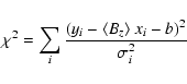
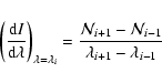

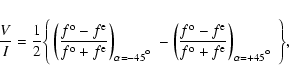

![\begin{displaymath}\begin{array}{rcl}
\sigma^2\left[(V/I)\right] & = &
\left(\l...
...rm e}} }\right)_{\alpha = +45\hbox{$^\circ$ }}. \\
\end{array}\end{displaymath}](/articles/aa/full/2006/17/aa4223-05/img83.gif)
![\begin{displaymath}\sigma^2\left[(V/I)\right] = \frac{1}{4m~\mathcal{N}}\cdot
\end{displaymath}](/articles/aa/full/2006/17/aa4223-05/img88.gif)
 \simeq 8 \times 10^{-4}\ \frac{1}{\sqrt{m}}\cdot
\end{displaymath}](/articles/aa/full/2006/17/aa4223-05/img104.gif)
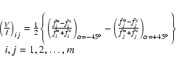
![\begin{displaymath}\overline{(V/I)} =
\sum_{ij} (V/I)_{ij}\; \sigma^{-2}[(V/I)_{ij}]\; /\;
\sum_{ij} \sigma^{-2}[(V/I)_{ij}] ,
\end{displaymath}](/articles/aa/full/2006/17/aa4223-05/img115.gif)
![\begin{displaymath}
\left\{\sigma^2\left[\overline{(V/I)}\right]\right\}' \simeq
\frac{1}{m}\sigma^2\left[(V/I)\right] .
\end{displaymath}](/articles/aa/full/2006/17/aa4223-05/img119.gif)
![\begin{displaymath}
\left\{\sigma^2\left[\overline{(V/I)}\right]\right\}'' \sim...
...rac{1}{m^2(m-1)} \sum_{ij} [(V/I)_{ij} - \overline{(V/I)}]^2 .
\end{displaymath}](/articles/aa/full/2006/17/aa4223-05/img120.gif)
![\begin{displaymath}\vert \ensuremath{\langle B_z\rangle}\vert / \sigma\left[\ensuremath{\langle B_z\rangle}\right] \ge 3 \\
\end{displaymath}](/articles/aa/full/2006/17/aa4223-05/img122.gif)
![\begin{displaymath}\ensuremath{\langle B_z\rangle} '\ =
\sum_{ij} \ensuremath{\...
...sigma^{-2}\left[\ensuremath{\langle B_z\rangle} _{ij}\right]
.
\end{displaymath}](/articles/aa/full/2006/17/aa4223-05/img124.gif)
![\begin{displaymath}\vert \ensuremath{\langle B_z\rangle} '\ \vert / \sigma\left[\ensuremath{\langle B_z\rangle} '\right] \ge 3
\end{displaymath}](/articles/aa/full/2006/17/aa4223-05/img128.gif)


![$\displaystyle \ensuremath{\sigma^2[{\bar{v}}]} =
\left(\sum_{i=1}^n\sum_{j=1}^m...
...+
\ensuremath{\sigma^2[{\phip_j}]}\sum_{h=1}^n\sigma^{-2}_{hj}
\right)
\right].$](/articles/aa/full/2006/17/aa4223-05/img174.gif)
![\begin{displaymath}\ensuremath{\sigma^2[{\phim_i}]} =\ensuremath{\sigma^2[{\phip_j}]} =\sigma^2_{ij}/2=\sigma^2/2 ,
\end{displaymath}](/articles/aa/full/2006/17/aa4223-05/img175.gif)
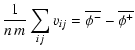

![\begin{displaymath}
s^2 =
\frac{1}{m\,n\,[2\,n\,m/(n+m)-1]}\;
\sum_{ij} \left( v_{ij} - \bar{v} \right)^2
,
\end{displaymath}](/articles/aa/full/2006/17/aa4223-05/img186.gif)