1 - Institut für Physik, Institutsbereich Geophysik, Astrophysik und Meteorologie, Universitätsplatz 5, 8010 Graz, Austria
2 - Astronomical Institute, Slovak Academy of Sciences, 05960 Tatranská Lomnica, Slovakia
3 - Kiepenheuer-Institut für Sonnenphysik, Schöneckstrasse 6, 79104 Freiburg, Germany

Abstract
Time series of 1D spectrograms are used to study the influence of the 5-min oscillations on intensity and velocity fields of different layers of the quiet solar photosphere. We study the continuum intensity field along with intensity and corresponding velocity patterns of the mid and upper photosphere, obtained from two Fe lines. Oscillations seem to dominate the intensity and velocity fields of the higher atmospheric layers. Our results confirm the fast decay of the granular intensity structure with height. From correlations of temperature structures at three different photospheric levels we conclude that there are rapid changes of the structures in the lower photosphere, which are valid for the duration of the time series, while for the upper levels changes of the stuctures are fainter and show significant periodic character. The velocity pattern, on the other hand, shows a periodic propagation through the photosphere. The tests of the influence of seeing conditions on the data are considered.

1 Introduction

Calculating correlations between characteristic quantities, such as intensity and velocity, can help to understand the physics of the solar granulation and the structure of the photosphere. The intensity structure is a reflection of the photospheric temperature structure. The intensity and velocity fields represent the granular pattern on the solar disk, which changes with increasing height in the photosphere. Also the relationship between intensity and velocity changes with height.

The aim of this paper is to study the variability of correlation coefficients with time due to the influence of the 5-min oscillations. With that we can study the change of amplitude and period of the oscillations with height, while additionally gaining insight on how oscillations can alter resulting correlation coefficients of single spectra or averages over short time series.

Many papers have been published considering the correlations between characteristic physical parameters. Various authors (e.g. Mattig et al. 1969; Canfield & Mehltretter 1973; Hanslmeier et al. 1990; Komm et al. 1990; Nesis et al. 1993) found a good correlation between continuum intensity and velocity. The good, but not perfect correlation was first thought to be due to the low resolution of the spectrograms used (Mattig et al. 1969), since they supposed the granular convection to be symmetric (bright regions correspond to upflows). Later it was found that the granular convection is asymmetric, which means that the maxima of intensity and velocity do not always coincide (Nesis et al. 1993). Gadun et al. (2000) used a multi-scale model based on 2D radiation hydrodynamics to predict correlations and their height dependance. They could confirm the good correlation between continuum intensity and velocity. Between residual intensity and velocity, they predicted an anticorrelation which decreases with height. Comparison with observations confirmed their theoretical results. Another possibility is to study correlations of the same quantity emerging from different photospheric heights. Hanslmeier et al. (1990, 2000) showed that a good correlation between the velocity patterns from different heights exists, even at differences of more than 300 km.

Many authors have drawn similar conclusions concerning the vertical structure of the photosphere. With many different methods (correlation analysis, coherence analysis), they all found a decrease of the granular intensity pattern with height. Above 170 km there should exist some non-convective, secondary structure (e.g. Nesis et al. 1988; Komm et al. 1990; Kucera et al. 1995; Krieg et al. 1999).

There have also been many attempts to make theoretical simulations of the granulation (e.g. Stein & Nordlund 1989; Steffen et al. 1989; Solanki et al. 1996; Steiner et al. 1998; Asplund et al. 2000; Ploner et al. 1999; Wedemeyer et al. 2004; Vögler et al. 2005). Gadun et al. (1999, 2000) also calculated theoretical correlation coefficients between parameters derived from their simulations.

Espagnet et al. (1995, 1996) investigated the connection between the 5-min oscillations and the granular pattern. They compared the coherence between line parameters of filtered and unfiltered data and could show the influence of the oscillations on the results. They found oscillatory cells with a size of 2-3 $^{\prime \prime }$ and a wide range of amplitudes. A typical period of about 5 min was found in the lower photosphere; in the higher layers the period decreased to about 3 min. They found an increase of the amplitude with height. Also Gadun et al. (1999) mentioned the importance of oscillatory motion, especially in the middle and upper photosphere. Khomenko et al. (2001) used a time series of spectrograms to investigate the connection between granulation and oscillations. They found that amplitudes, periods and phases of the oscillations are different above granules and the intergranulum.

Some theoretical models also try to simulate the granulation combined with oscillations. Gomez et al. (1987) investigated the influence of the 5-min oscillations on line profiles. They showed that the flanks of the line are affected differently by oscillatory motion.

Here, we focus on a quiet region in order to study the influence of the 5-min oscillations on intensity and velocity patterns at various heights in the photosphere.

2 Data and observations

The data used for this work consists of time series of spectrograms. They were recorded on April 28th 2000 with the German Vacuum Tower Telescope (VTT) (Schröter et al. 1985) at the Observatorio del Teide (Izaña, Tenerife). The recordings were carried out from 09:26:36 to 09:41:36 UT, targeting the quiet atmosphere almost in the center of the solar disk. The target was located near AR 8976. The slit of the Echelle spectrograph was oriented perpendicularly to the horizon, the slit width was $100~\mu{\rm m}$ , equivalent to 0.5 $^{\prime \prime }$ . The Adaptive Optics system of the NSO/SP was installed at the VTT for testing purposes; it helped greatly to compensate for seeing and guiding inaccuracies. The slit-jaw imaging system (Kentischer 1995) was used to record the exact position of the spectrograph slit on the solar disk, in particular the G-band filter of 9 Å bandpass centered at 4306 Å. This system was operated with the $1{\rm k}\times1{\rm k}$ 16 bit DALSA digital camera, an exposure time of 5 ms and a cadence of 2 frames per second was used. Two spectral regions were recorded simultaneously (around 4994.3 Å and 6456.4 Å) with two $2{\rm k}\times2{\rm k}$ 12 bit XEDAR XS-2048-A-12 CCD cameras using $2\times2$ pixel hardware binning. Here, the exposure time was 1 s. The time series consists of 300 spectra separated by 3 s. Spatial and spectral samplings are 0.125 $^{\prime \prime }$ per pixel and 2.4096 mÅ per pixel, respectively.

All spectra were then photometrically reduced using the precise reduction procedure of Wöhl et al. (2002), which considers the temporal variation of the flat field. High frequency noise was removed by Gaussian filtering (Gray 1976). The polynomial approximation of the dispersion was determined from the averaged spectra with the wavelength data of Moore et al. (1966). The average line position of all spectra was used to adjust the zero point of the wavelength scale. The intensity scale was normalized using the quasi-continua and considering their relation to the true continuum level (Neckel 1999). The center-to-limb darkening was removed. The spectra were normalized according to the mean continuum value of all spectra. The spectral line parameters were determined for all lines and all spectra, such as the continuum intensity, the residual intensity and the Doppler velocity. The quality of the spectra, indicated by the relative rms contrast of the continuum intensity, is displayed in Fig. 1.

The data used in the next section do not include the whole spectrogram. For each of the 300 spectra of this 15 min time series, the variations of the line parameters along the slit were calculated. 950 values along the slit are used, this corresponds to about 120 $^{\prime \prime }$ on the solar disk. Here, the line parameters continuum intensity I, residual intensity r and Doppler velocity v are used. The velocity is given in km s^-1 and is negative for upflows and positive for downflows, with the mean position of the line as the reference.

Table 1 is a collection of some important characteristics of the chosen spectral lines, such as the element, the wavelength $\lambda$ , the excitation potential EP (both taken from Kurucz's CD-ROM) and the equivalent width $W_{\lambda}$ (taken from Liege atlas, Delbouille et al. 1973). Also given are the effective line formation heights for the line central depth $H_{\rm d}$ and the geometrical height $H_{\tau}$ at line center optical depth $\tau_{\lambda0}=\tau^{{\rm C}+{\rm L}}_{\lambda0}=1.0$ (C...continuum, L...line), both calculated with two different models. $H_{\rm d}$ was calculated with the depression contribution function. The models used for the height estimation were the MACKKL model (Maltby et al. 1986) and a 1D model which was obtained by spatial and temporal averaging of 2D models (e.g. Gadun et al. 1999, 2000). Since 2D models do not consider the chromospheric heating, they can produce incorrect formation heights for some lines.

$\begin{figure} \par\includegraphics[width=8.4cm,clip]{3082fig1.eps} \end{figure}$	Figure 1: The variation of the relative rms contrast of the continuum intensity during the time series. The wavelength range used was centered at 4993.12 Å and the slit length used for the calculation was 65 $^{\prime \prime }$ .
Open with DEXTER

Table 1: Characteristics of the selected spectral lines: Element, wavelength, excitation potential and estimated formation heights obtained with two models.

3 Results

We study the influence of oscillations on correlations between spectral line parameters. The main idea is to investigate the temporal variations of the correlations (Sect. 3.3), instead of just calculating the commonly used mean values. To compare the results of this paper with others, the averages over the whole time series are given (Sect. 3.4). First, it is necessary to take a closer look at the temporal-spatial maps of the used data.

3.1 Temporal-spatial maps

The temporal evolution of the granulation can be investigated with temporal-spatial maps. Note that in the following figures the contrast has been enhanced to emphasize the details of the structures. Thus, the maximum and minimum values on the scales are not the respective largest and smallest values of the original data array. From the simultaneously recorded slit-jaw images we see that some small spots are located on one side of the slit, as well as two pores directly on the slit.

Figure 2 displays the temporal-spatial map of the continuum intensity. Since the slit spans over 100 $^{\prime \prime }$ , only the largest granules can be distinguished clearly. The dark region at 70-82 $^{\prime \prime }$ is caused by the above-mentioned pores which could be seen on the slit-jaw images. The horizontal stripes (e.g. after 100 s, 400 s, 700 s) are due to worse seeing conditions (see also Fig. 1).

The temporal-spatial map of the residual intensity of the mid-photospheric Fe II line (Fig. 3, upper panel) has a similar structure, but bright and dark regions seem inverted compared to the continuum intensity. The formerly dark pores appear bright at this photospheric height. The temporal-spatial map of the residual intensity of the even higher forming Fe I line (Fig. 3, lower panel) does not look similar to the previous figures. One can see that the convective granular pattern has disappeared at this height and is replaced by some other faint structure, but the active regions can still be seen clearly as bright lanes.

In both temporal-spatial maps of the Doppler velocities (Fig. 4) one can see that the velocity fluctuations are reduced by the magnetic field of the pores and the anomalous granulation in the region 60-90 $^{\prime \prime }$ . The velocity of the higher Fe I line (Fig. 4, lower panel) does not show the typical structure of the granulation any longer, but is dominated by a different pattern caused by oscillatory motions. In the velocity map of the lower Fe II line (Fig. 4, upper panel) there is a mixture of granular and oscillatory structure. While in the continuum and lower residual intensity maps only the pores can be distinguished clearly, in the higher residual intensity and both velocity maps also the surrounding anomalous granulation is visible. The normal granulation of a quiet region can be seen between 0 $^{\prime \prime }$ and almost 60 $^{\prime \prime }$ in all temporal-spatial maps.

In the present paper we are interested in relations between the line parameters of a quiet region on the solar disk. Therefore, we only use data in the range of 0-55 $^{\prime \prime }$ (corresponding to 440 values along the slit) for the following calculations of the correlation coefficients.

$\begin{figure} \par\includegraphics[width=8.4cm,clip]{3082fig2.eps} \end{figure}$	Figure 2: Temporal-spatial map of the continuum intensity. The horizontal stripes of lower intensity contrast are due to seeing (see Fig. 1).
Open with DEXTER

$\begin{figure} \par\includegraphics[width=8.4cm,clip]{3082fig5.eps} \end{figure}$	Figure 5: Comparison of the rms fluctuations of the continuum intensity (same as Fig. 1) with the temporal variations of correlations to determine the influence of seeing.
Open with DEXTER

3.2 The influence of seeing on correlation coefficients

We also investigated the influence of seeing on the calculated correlation coefficients. Therefore, correlations between the rms fluctuation of the continuum intensity (Fig. 1), which represents seeing, and our calculated variations of the correlations were determined. An example of this comparison is given in Fig. 5. The results can be found in Table 2. This correlation is always higher for parameters of the lower Fe II line (index 1), since the structural patterns of the lower line (upper panels in Figs. 3 and 4) are smaller and are therefore more sensitive to seeing. So the short time variations in our results should be due to seeing. The correlation between continuum and residual intensity of the Fe II line (r₁) seems to be most strongly affected by seeing, whereas the weakest effect is found for the correlation between continuum intensity and higher velocity (v₂). Figure 6 therefore displays the scatterplot of these two correlations versus the rms fluctuations. For the $\left\langle I,r_{1}\right\rangle$ -correlation we see that for worse seeing the anticorrelation decreases and we find an even distribution for the $\left\langle I,v_{2}\right\rangle$ -values.

Table 2: The correlation of the rms fluctuation of the continuum intensity with our resulting correlations. Generally, the correlations are higher for parameters of the lower forming line (index 1) indicating a larger seeing influence.

$\begin{figure} \par\includegraphics[width=8.4cm,clip]{3082fig6.eps} \end{figure}$	Figure 6: Temporal variation of two correlation coefficients versus the rms of the continuum fluctuations (Asterisks: $\left\langle I,r_{1}\right\rangle$ , triangles: $\left\langle I,v_{2}\right\rangle$ ).
Open with DEXTER

3.3 Temporal variation of correlation coefficients

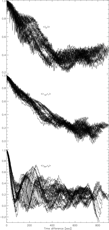
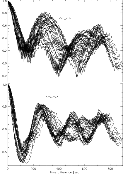
Figures 7 and 8 display spatial correlations at zero lag between one temporal realization of a process and the subsequent ones, which we term autocorrelations hereafter, of the used line parameters. A quantity of the initial spectrum of the time series is correlated with the same quantity of all subsequent spectra. These correlations start, of course, with 1 and usually decrease with increasing time difference between the spectra until all memory of the initial structure is lost. To take into account a possible dependance of the results on the starting spectrum, we display the results for each second (i.e. every 6 s) of the first 70 spectra ( $\sim$ 200 s) in the following figures.

The autocorrelations of the intensities are displayed in Fig. 7. The autocorrelations of the continuum intensity I show a general decrease with time for all starting spectra. After about 500 s, the correlations start to oscillate around a mean value of 0.4. The autocorrelations of the residual intensity of the lower line (r₁) show a quite linear decrease with increasing time difference; results from different starting spectra are even more similar than for the continuum intensity. The autocorrelations of the residual intensity of the higher line (r₂) behave differently to the lines mentioned. The curves from all starting spectra show a rapid drop of correlation in less than 100 s. For the rest of the time series, the correlations have the character of a damped oscillation for all curves, but the amplitude and period seem to depend on the starting spectrum.

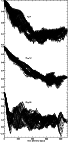$\begin{figure} \resizebox{\hsize}{!}{\includegraphics{3082fg7a.eps}}\par\resizeb... ...fg7b.eps}}\par\resizebox{\hsize}{!}{\includegraphics{3082fg7c.eps}} \end{figure}$	Figure 7: The autocorrelations of the intensities I (continuum), r₁ (Fe II) and r₂ (Fe I) with increasing time difference. Each second of the first 70 spectra was taken as a starting spectrum.
Open with DEXTER

$\begin{figure} \resizebox{\hsize}{!}{\includegraphics{3082fg8a.eps}}\par\resizebox{\hsize}{!}{\includegraphics{3082fg8b.eps}} \end{figure}$	Figure 8: The autocorrelations of the velocities v₁ (Fe II) and v₂ (Fe I) with increasing time difference. Each second of the first 70 spectra was taken as a starting spectrum.
Open with DEXTER

The autocorrelations of the velocities (Fig. 8) are different compared to those of the intensities. Both clearly show oscillatory characteristics. The correlations of the velocity structure at the formation level of the Fe II line (v₁) drop to a minimum in the region of 150 s, then show oscillatory behavior with large amplitudes for all starting spectra. There is a shift of period of these oscillations depending on the starting spectrum. The overall correlation moves to a lower value with increasing time difference. The autocorrelations of the velocity of the higher line (v₂) bear more resemblance to the results of the higher residual intensity. There is also a rapid drop of correlation reaching a quite significant anticorrelation of -0.7 after a time difference of about 100 s. Then oscillations with lower amplitudes take place. They are not all in phase, but compared to the residual intensity of the same photospheric level, a general structure is visible more clearly.

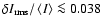
The following figures display spatial correlations at zero lag between two quantities as a function of the temporal realizations, which we term cross correlations hereafter. The horizontal bars in the upper/lower parts of the following figures indicate times of worse seeing conditions ( $\delta I_{{\rm rms}}/\left\langle I\right\rangle\la0.038$ ). The crosscorrelations were calculated for original and detrended data, but since we found no significant discrepancies, the results for the original data are presented here.

Figure 9 displays this crosscorrelation between the various intensities. For the correlation between continuum and residual intensity of the lower line, we find a medium anticorrelation which is heavily influenced by seeing effects (see Sect. 3.2) and does not show any significant periodic structure. The correlation between the two residual intensities is positive and the influence of oscillations is clearly visible. This correlation fluctuates around the value of 0.2 with a large amplitude ( $\sim$ 0.5) and a period of about 200 s. The correlation between continuum intensity and higher residual intensity represents a mixture of the other correlations. On the one hand, there is a medium anticorrelation with some seeing influence comparable to the $\left\langle I,r_{1}\right\rangle$ -correlation, on the other hand it also shows oscillations with a period of about 200 s, which are in antiphase with the $\left\langle r_{1},r_{2}\right\rangle$ -correlation.

$\begin{figure} \par\includegraphics[width=8.4cm,clip]{3082fig9.eps} \end{figure}$	Figure 9: The temporal variation of the crosscorrelation between continuum and residual intensities for the Fe II line (solid) and the Fe I line (dotted) and between both residual intensities (dashed). Horizontal bars indicate times of worse seeing.
Open with DEXTER

$\begin{figure} \par\includegraphics[width=8.4cm,clip]{3082fg10.eps} \end{figure}$	Figure 10: The temporal variation of the crosscorrelation of the velocity of the Fe I line with continuum intensity (solid), residual intensity of Fe II (dashed), and residual intensity of Fe I (dotted). Horizontal bars indicate times of worse seeing.
Open with DEXTER

$\begin{figure} \par\includegraphics[width=8.4cm,clip]{3082fg11.eps} \end{figure}$	Figure 11: The temporal variation of the crosscorrelation between both velocities. Horizontal bars indicate times of worse seeing.
Open with DEXTER

The crosscorrelations between the velocity of the Fe I line and all intensities (Fig. 10) shows temporal variations with large amplitudes in all cases. For the correlation with the continuum intensity we find a low anticorrelation oscillating with a period of about 250 s (minima after 100 s, 350 s, 600 s and 850 s). In the maximum after $\sim$ 250 s, the correlation is positive, whereas in the other maxima (450 s and 750 s) the correlation is zero. The correlation with the residual intensity of the lower Fe II line changes between negative and positive correlation during the first half of the time series with positive maxima after about 150 s and 300 s and a minimum after about 250 s. In the second half, the correlation remains mainly positive with maxima at about 700 s and 850 s, and minima with approximately zero correlation at about 600 s and 750 s. This correlation is in antiphase to the continuum intensity correlation, except between 450 s, and 750 s, where they are in phase. The correlation between velocity and residual intensity of the Fe I line is low and even reaches a medium anticorrelation of -0.35 in the pronounced minimum between 200 and 250 s. In the other minima, the correlation is approximately zero. Large maxima are found after 150 s and 350 s, then follow smaller maxima after 600 s, 750 s and 850 s. This correlation also changes between being in phase or antiphase with the continuum intensity. It is in antiphase during the first 450 s and from 650 s to 800 s, all other times they are in phase. The correlations with the two residual intensities are in phase up to 480 s, then in antiphase until 800 s, and then again in phase.

The crosscorrelations of both the continuum and lower residual intensities with the velocity of the Fe II line (not shown here) reveal variations with an amplitude of about 0.5 due to the 5-min oscillations around mean values of about -0.67 for the continuum and 0.2 for the residual intensity, respectively. These variations are in antiphase during the first 600 s, then they are in phase.

Figure 11 shows the temporal variation of the crosscorrelation between the velocities of both lines. Considering that the two lines are formed in atmospheric layers separated by more than 300 km, the correlation is still good, fluctuating around a mean value of 0.6. The influence of the 5-min oscillations is clearly visible, and the amplitude of the resulting fluctuation is quite large ( $\sim$ 0.45). The period is about 300 s, which is longer than the period found for the correlation between the residual intensities of the corresponding photospheric levels in Fig. 9.

We tested the significance of the crosscorrelations with the Monte Carlo method. We calculated the correlations for 1000 realizations of randomized space-time arrays of the line parameters. The levels above (or below in the case of anticorrelation) which 10% of the randomized correlation values lie are given in Table 3.

Table 3: Levels of significance (10%) for all crosscorrelations. For coefficients fluctuating around zero, upper and lower levels are given.

3.4 Mean correlation coefficients

For easier comparison with other results, some temporally averaged correlation coefficients are collected in Table 4. Results from some other papers are also given. The values of Canfield & Mehltretter (1973) are from lines with respective formation heights of 160 km and 500 km. The values of Hanslmeier et al. (1990) are from lines at about 135 km and 500 km, respectively. The comparative value for the $\left\langle v_{1},v_{2}\right\rangle$ -correlation was chosen for a height difference of 300 km.

Table 4: (a) Some averaged correlation coefficients with standard deviations; comparative values from (b) Canfield & Mehltretter (1973) and (c) Hanslmeier et al. (1990).

4 Discussion and conclusion

The results for the averaged values of the correlation coefficients (Table 4) show that the mean values are not capable of representing the real physical situation, because the 5-min oscillations have a strong influence. The correlation coefficients can fluctuate strongly with amplitudes of over 0.4 during a time series, and the amplitudes of these fluctuations are larger for the higher forming line. While our results for $\left\langle I,v\right\rangle$ -correlations are in good agreement with the ones of Canfield & Mehltretter (1973), large discrepancies are found for the $\left\langle I,r\right\rangle$ -correlations. Whereas we find a medium anticorrelation for both lines, Canfield & Mehltretter (1973) found almost no correlation at these heights, and Hanslmeier et al. (1990) found a medium positive correlation for the lower and no correlation for the higher line. As can be seen from the temporal evolution of the correlation coefficients, this can be a problem when using single spectra or very short time series. Our results are also in agreement with the theoretical correlations of Gadun et al. (2000), which were derived from a 2D multi-scale model. They also compared their model results with observations and were able to reproduce them quite well; some discrepancies are supposed to be due to the spatial limitation of the model, the Cartesian approach, as well as the close-to-laminar treatment of the medium.

The influence of oscillations can be seen in the temporal-spatial maps. The lower panels in Figs. 3 and 4 (parameters of the higher line) show a wave structure which has nothing in common with the typical granular pattern. The time-slice diagrams of Espagnet et al. (1996) display the granular structure separated from the structure of the 5-min oscillations. The oscillatory structure shows some similarity to the lower panels of Figs. 3 and 4 of this paper. It can be concluded that the oscillatory structure is dominant at this height and lies over other possible structures. Also, the continuum intensity map shows mainly the largest granules, which are long-lived and survive almost the entire time series. The map of the velocity of the lower line shows shorter granular structures. This is in accordance with the findings of Nesis et al. (2002), who found the well established lifetime of 7-9 min for granular intensity structures in the continuum intensity map and a shorter dynamical time of granular velocity structures of 2-5 min. Our results also confirm the temperature reversal in the overshooting layer, which has been predicted by various theoretical models (e.g. Steffen et al. 1989; Stein & Nordlund 1989) and was also confirmed by observations (e.g. Espagnet et al. 1995).

The autocorrelations of the intensity patterns from three different photospheric levels show quite different behavior (Fig. 7). Whereas some fluctuations of the continuum intensity seem to represent the lifetime of the granulation, the decrease of the lower residual intensities is more linear. The autocorrelation of the residual intensity of the higher line behaves completely differently. There are large fluctuations with decreasing amplitude suggesting similarity to a damped oscillation. However, the period and the actual amplitude depend on the choice of the starting spectrum. The rapid drop of the correlation to zero, or even slightly negative values, in less than 100 s seems to be independent of the starting spectrum. The autocorrelations of the velocities of both photospheric heights clearly show the properties of the 5-min oscillations (Fig. 8). Even after larger time differences, the local maxima reach almost the same values as the first maximum indicating a periodic propagation of the velocity field through the photosphere, as was also found by Espagnet et al. (1995). The autocorrelation of the higher line's velocity shows some similarity to the residual intensity of the same level, thus representing non-granular structure at this photospheric height (see Figs. 3 and 4).

The anticorrelation of intensity structures (representing roughly the temperature behavior) between continuum and mid-photospheric Fe II line (Fig. 9) are again in agreement with Espagnet et al. (1995) where it was shown that intensity structures lose their identity rapidly with height already in the lower photosphere. The oscillatory character of the correlation coefficient is mainly caused by changes of seeing (see Sect. 3.2). The correlation between temperature structures of the two photospheric levels of Fe II and Fe I has a real oscillatory character. This means that temperature structures at these two photospheric heights are periodically similar and dissimilar. In accordance with the relative behavior of the $\left\langle I,r_{1}\right\rangle$ and $\left\langle r_{1},r_{2}\right\rangle$ -correlations, the $\left\langle I,r_{2}\right\rangle$ -correlation reflects the oscillatory behavior of temperature structure occurrence between the mid and high photosphere as well as the mean value of the $\left\langle I,r_{1}\right\rangle$ -correlation. The 200 s-period of the $\left\langle I,r_{2}\right\rangle$ -correlation confirms the decrease of the period of the 5-min oscillations to about 3 min in higher layers, as found by Espagnet et al. (1995, 1996). From the three correlations of temperature structures at different photospheric levels we can generally conclude that there are rapid changes of the structures in the lower photosphere, which are valid for the whole time series, while for the upper levels, changes of the structures are fainter and show significant periodic behavior.

Variations of the anticorrelation between the Doppler velocity of the upper forming line and the continuum intensity are strongly influenced by the 5-min oscillations (Fig. 10). Both correlations of the Doppler velocity of the upper forming line with residual intensities of both lines are in phase. They demonstrate the reversal of the intensity field at the levels where the particular lines are formed, as was found by Kucera et al. (1995). The phase shift of the correlations shows the propagation of the 5-min oscillations through the solar photosphere.

The correlation between the velocity patterns of the mid and high photosphere (Fig. 11) changes periodically in time reaching a high degree of selfsimilarity every $\sim$ 300 s. This appears when the power of 5-min oscillations of the lower line's velocity (Fig. 4, upper panel) is maximal and dominates the power of the velocity signal coming from the granular pattern.

Our results show that the seeing effect influences the correlation coefficients. The influences depend on the line parameters investigated and the formation heights of the photospheric line. We find a stronger seeing influence for correlations with parameters of the lower line (e.g. solid curve in Fig. 9). The reason for this could be a general dependence of the correlation coefficients on the typical sizes and the contrast of 2D structures. As can be seen in Figs. 2-4, the structures are smaller for continuum intensity and parameters of the lower line compared to parameters of the higher line. Velocity structures are also larger than intensity structures. This is exactly what we see in our figures: correlations with the velocity (e.g. Figs. 8 and 10) are less influenced by seeing (of course, depending on what other parameters are involved) than correlations with the residual intensity (e.g. Fig. 9). For correlations with parameters from the higher line, the result is always smoother than the same correlation for the lower line (e.g. Figs. 9 and 10). The reason for a lower contrast in the spectra for stronger seeing is that the scattering of light falling into the slit from surrounding areas (and vice versa) is more efficient. If 2D intensity/velocity structures are smaller and/or the contrast of the structures is higher, then the correlation coefficient is more sensitive to seeing.

Thus, we find a disappearance of the typical granular intensity structures at lower heights, while the velocity structures propagate periodically through the whole photosphere. In the upper photosphere, intensity and velocity fields are dominated by oscillatory structures, as indicated by periodic changes of the correlation coefficients.

Influence of the 5-min oscillations on solar photospheric layers

I. Quiet region