T. Buchert1,2,3 - A. Domínguez4,5,6
1 - Arnold Sommerfeld Center for Theoretical Physics, Ludwig-Maximilians-Universität,
Theresienstr. 37, 80333 München, Germany
2 -
Theory Division, CERN, 1211 Genève 23, Switzerland
3 -
Observatoire de la Côte d'Azur, Lab. G.D. Cassini,
BP 4229, 06304 Nice Cedex 4, France
4 -
Max-Planck-Institut für Metallforschung,
Heisenbergstr. 3, 70569 Stuttgart, Germany
5 -
Institut für Theor. und Angew. Physik,
Univ. Stuttgart, Pfaffenwaldring 57, 70569 Stuttgart, Germany
6 -
Física Teórica, Univ. Sevilla, Apdo. 1065, 41080 Sevilla, Spain
Received 16 February 2005 / Accepted 7 March 2005
Abstract
The notion of adhesion has been advanced for
the phenomenon of stabilization of large-scale structure
emerging from gravitational instability of a cold medium.
Recently, the physical origin of adhesion has been identified:
a systematic derivation of the equations of motion for the
density and the velocity fields leads naturally to the
key equation of the "adhesion approximation'' - however, under
a set of strongly simplifying assumptions.
In this work, we provide an evaluation of the current status of
adhesive gravitational clustering and a clear explanation of the
assumptions involved. Furthermore, we propose systematic
generalizations with the aim to relax some of the simplifying
assumptions. We start from the general Newtonian evolution
equations for self-gravitating particles on an expanding
Friedmann background and recover the
popular "dust model'' (pressureless fluid), which breaks down
after the formation of density singularities; then we investigate,
in a unified framework,
two other models which, under the restrictions referred to above,
lead to the "adhesion approximation''. We apply the Eulerian and
Lagrangian perturbative expansions to these new models and,
finally, we discuss some non-perturbative results that may serve as
starting points for workable approximations of non-linear structure
formation in the multi-stream regime.
In particular, we propose a new approximation that includes, in
limiting cases, the standard "adhesion model'' and the Eulerian as well as
Lagrangian first-order approximations.
Key words: gravitation - methods: analytical - cosmology: theory - cosmology: large-scale structure of Universe
The present work aims to push analytical modeling of structure formation into a regime that may be placed between the formation epoch of large-scale structure and the onset of virialization of gravitationally bound objects. Phenomenologically, this regime is characterized by a stabilization of structures that formed out of gravitational instability of a cold medium. The physical origin of this adhesive clustering effect is the balance of gravitational forces and dynamical stresses in collisionless matter. The latter arise from a subsequently establishing multi-stream hierarchy within collapsing high-density regions. Although multi-stream forces tend to disperse structures, the resulting effect together with gravity tends to stabilize them. This regime is summarized by the term non-dissipative gravitational turbulence advanced by Gurevich & Zybin (1995). The models we investigate are a focus of current research, since efforts to simulate Hubble volumes of the Universe and to understand galaxy halo formation are faced within a single approach. However, we take a more conservative point of view to understand the evolution of structure on galaxy cluster scales (for a recent theoretical attempt to address halo structure within kinetic theory see Ma & Bertschinger 2004).
The current status of analytical models concerning large-scale structure formation may be centred on Zel'dovich's approximation together with its foundations (the Lagrangian perturbation theory) and optimizations using filtering techniques for initial perturbation spectra (Zel'dovich 1970, 1973; Shandarin & Zel'dovich 1989; Buchert 1989, 1992; Melott 1994; Bouchet et al. 1992, 1995; Sahni & Coles 1995; Buchert 1996; Ehlers & Buchert 1997). These schemes are capable of modeling the evolution of generic spectra including Cold-Dark-Matter cosmogonies down to galaxy cluster scales (Bouchet et al. 1995; Buchert et al. 1994; Melott et al. 1995; Weiß et al. 1997; Hamana 1998). Above these scales the optimized Lagrangian schemes roughly reproduce the results of N-body simulations. Since the exact solution is not known, we seek agreement between the two modeling techniques used. Below these scales, both techniques tend to fail as a result of both poorly understood physics and poor resolution power, respectively. Agreement between N-body simulations and simple solutions of Lagrangian perturbation schemes may be considered as supporting analytical models, but they could as well be considered as a drawback of N-body simulations given the simplicity of the analytical approximations compared with the complexity of non-linear self-gravity. A deeper understanding of structure formation below galaxy cluster scales may require more than improving spatial resolution. The use of N-body computing in cosmology is possibly overstated as is indicated by the differing results obtained when using different N-body codes on the scales of interest (Melott et al. 1997; Splinter et al. 1998). Furthermore, particular features show that caution is in order: (i) the validity of the mean field approximation for the gravitational field strength that is commonly used is questionable, especially on the scales of galaxy halos; (ii) the possible emergence of soliton states (Götz 1988) that arise as a result of the non-linear interaction between gravity and pressure-like forces; solitons have special stability properties and may dominate large-scale structure at late times; (iii) the behavior of the gravitational field strength near high-density regions: from a generic integral of the field equations (Buchert 1993a, Sect. 6.1) one clearly infers proportionality of the field strength and the density, whereas Lagrangian perturbation schemes (in the regime where they match N-body runs) show smooth and moderately increased field strengths when crossing high-density regions. In the extreme case of infinite resolution, Zel'dovich's approximation produces caustics in the density field, whereas the field strength remains smooth, although it should blow up at caustics; whether N-body codes treat this correctly is questionable in view of the strongly varying fields on the spatial as well as temporal resolution scales.
In this situation, analytical models that are capable of accessing non-linear scales should be further explored. This task is not easy, since - as explained above - such models may not be fully guided by comparisons with N-body results. The pioneering model for adhesive clustering has been built in view of the shortcomings of Zel'dovich's approximation predicting structure decay after their formation: a Laplacian forcing has been added ad hoc to the evolution equation for the peculiar-velocity. Such a force has the right property of holding structures together after their formation and, moreover, the model can be solved exactly in terms of known solutions of the 3D Burgers' equation (Gurbatov et al. 1989; Weinberg & Gunn 1990; Kofman et al. 1990, 1992, 1994; see also: Gurbatov et al. 1983, 1985, 1991). The phenomenon of non-dissipative gravitational turbulence is mimicked by the so-called "burgulence'' (Frisch & Bec 2001) and roughhewned into an "effective viscosity''. However, the performance of the "adhesion approximation'' does not dramatically improve the Lagrangian perturbation schemes, if the latter are subjected to optimization techniques as mentioned above: even for a strongly hierarchical power spectrum (power law index of n = -1) the optimized Lagrangian schemes yield better cross-correlation statistics for the density fields, compared with numerical simulations (Buchert 1999). However, comparisons have been conducted only on the level of large-scale structure (e.g., Sahni et al. 1994 investigate the evolution of voids); the role that the "adhesion approximation'' could play on subcluster scales has not been explored. Other proposals to analytically model the weakly non-linear regime tried to improve the performance for large-scale structure, e.g. "freezing'' the initial streamlines of the fluid keeping the velocity potential constant (so-called "Frozen Flow Approximation'', Matarrese et al. 1992), or treating the gravitational potential as constant ("Frozen Potential Approximation'', Brainerd et al. 1993; Bagla & Padmanabhan 1994). However, these approximations, by their nature, are unable to model a realistic evolution beyond the epoch when the time-dependence of the velocity or the potential is important, cf. the systematic comparison of different models carried out by Sathyaprakash et al. (1995).
Lying at the physical core of the problem of covering multi-streaming, the "adhesion approximation'' is a promising model due to a strong support given to it by Buchert & Domínguez (1998): a Laplacian forcing appears naturally in a physical description of adhesive gravitational clustering and the "adhesion approximation'' can be derived on the basis of a set of - however, strongly simplifying - assumptions. The Laplacian forcing does not represent a true viscosity, it arises by combining the gravitational field equations with a dynamical pressure gradient due to multi-stream stresses. Consequently, momentum is conserved and energy is not lost: the model is time-reversible. Multi-streaming implies a reshuffling of energy components: bulk kinetic energy is transformed into internal kinetic energy, and the gravitational potential energy of a high-density region gradually dominates over the tidal interaction with its environment, thus effectively isolating the system and - in idealized cases - establishing a dynamical equation of state as a relation between gravitational potential energy and internal kinetic energy.
This reasoning can be made mathematically precise by deriving the
equations of motion for the coarse-grained (or filtered)
density and velocity fields. Given a smoothing length L, the system
is divided into the degrees of freedom of the scales above and below L, respectively.
The evolution of the smoothed density and velocity fields is in
general dynamically coupled to the degrees of freedom below L.
The standard "dust model'' is recovered by
assuming that the dynamical effect of this coupling is negligible.
When the "dust model'' develops singularities, this assumption
breaks down, and an improved model has to be used that
accounts for multi-streaming and the coupling to the small-scale
degrees of freedom. The model introduced by Buchert & Domínguez (1998),
which we call the Euler-Jeans-Newton ("EJN'') model, identifies
the main source of the corrections to "dust'' as the gravitational
multi-stream (GM) effect. This gives rise to a stress tensor of
purely kinetic origin - as in an ideal gas - which is added to
the large-scale gravity already considered by the "dust model''. This
stress may be idealized in the "EJN model'' phenomenologically as
isotropic, and modelled with a pressure
![]() depending only
on the density
depending only
on the density ![]() ,
i.e. a dynamical equation of state.
,
i.e. a dynamical equation of state.
Numerical tests (Domínguez 2003; Domínguez & Melott
2004) show that a polytropic equation of state,
![]() in a certain range of densities is
characteristic for a variety of initial conditions.
The "anomaly''
in a certain range of densities is
characteristic for a variety of initial conditions.
The "anomaly'' ![]() measures the deviations from the naive virial prediction
measures the deviations from the naive virial prediction
![]() ,
depends itself on initial conditions
(
,
depends itself on initial conditions
(![]() ranges from 0 to 1 as the small-scale power is reduced),
and can be assigned to the fact that
the fluid elements are not isolated and in a stationary state,
as required when deriving
ranges from 0 to 1 as the small-scale power is reduced),
and can be assigned to the fact that
the fluid elements are not isolated and in a stationary state,
as required when deriving
![]() from the virial theorem.
An exact integral of the form
from the virial theorem.
An exact integral of the form
![]() can be
deduced theoretically under certain strong assumptions
(Buchert & Domínguez 1998).
can be
deduced theoretically under certain strong assumptions
(Buchert & Domínguez 1998).
Recent developments of the "EJN model'' concern the Lagrangian linear regime (Adler & Buchert 1999), where solutions can be found by extrapolating known results of the Eulerian linear regime; the Lagrangian scheme has been developed to second order (Morita & Tatekawa 2001; Tatekawa et al. 2002) and recently to third order (Tatekawa 2005); numerical tests employing N-body and hydrodynamical simulations have been conducted by Tatekawa (2004a,b).
While the foundations of the "EJN model'' can be derived on the basis of
the velocity moment hierarchy
of the commonly employed Vlasov-Poisson system,
its practical implementation needs (phenomenological) closure conditions to
truncate the hierarchy.
An attempt to systematically go beyond phenomenology is the Small-Size Expansion
("SSE'') introduced by Domínguez (2000). The mode-mode coupling in the
equations for the fields smoothed over the scale L is estimated under the
assumption that the most important contribution to this coupling
comes from inter-mode coupling at scales ![]() L.
The systematic nature of this scheme is due to a formal expansion of this
coupling in powers of L.
The "dust model'' is recovered as the lowest order term
(formally setting L=0). The corrections also yield a Laplacian forcing
as well as the "adhesion model'' under certain simplifying assumptions.
However, the corrections account not only for the GM effect like the
"EJN model'', but also for the gravitational influence of the density
inhomogeneities on scales below L: the stress tensor has an additional
potential-energy contribution that can be viewed as a correction to
the mean field approximation for the gravitational field-strength and
also provides a Laplacian forcing, although
subdominant relative to the one due to the GM effect. This effect may become
dominant if one aims to describe structure evolution on galaxy halo scales.
The stress tensor in the "SSE model'' is also a source of
vorticity by tidal torques and shear stretching. This has been studied recently
with the Eulerian perturbation expansion (Domínguez 2002).
L.
The systematic nature of this scheme is due to a formal expansion of this
coupling in powers of L.
The "dust model'' is recovered as the lowest order term
(formally setting L=0). The corrections also yield a Laplacian forcing
as well as the "adhesion model'' under certain simplifying assumptions.
However, the corrections account not only for the GM effect like the
"EJN model'', but also for the gravitational influence of the density
inhomogeneities on scales below L: the stress tensor has an additional
potential-energy contribution that can be viewed as a correction to
the mean field approximation for the gravitational field-strength and
also provides a Laplacian forcing, although
subdominant relative to the one due to the GM effect. This effect may become
dominant if one aims to describe structure evolution on galaxy halo scales.
The stress tensor in the "SSE model'' is also a source of
vorticity by tidal torques and shear stretching. This has been studied recently
with the Eulerian perturbation expansion (Domínguez 2002).
In the present work the "dust'', the "EJN'' and the "SSE'' models will be presented in a unified framework, as different closure approximations to a hierarchy of equations, and a clearcut description of the weakly non-linear regime of adhesive gravitational clustering will be offered. It is expected that the gravitational multi-stream process (GM-effect for short) as well as stresses arising from corrections to the mean field approximation may help to establish the stationary configurations that are usually studied in stellar systems theory, where "virialized objects'' are, however, considered as isolated entities.
Section 2 applies the coarse-graining method to cosmological structure formation in the phase space of N particles, resulting in a continuum description which features the Vlasov dynamics as a subcase. Section 3 describes the resulting fully non-linear evolution equations for the density and peculiar-velocity fields in Eulerian space and summarizes the assumptions that reduce the general problem to the key equation of the "adhesion approximation''. Section 4 reviews the application of the Eulerian perturbative expansion and Sect. 5 that of the Lagrangian perturbative expansion. Section 6 presents new results beyond the perturbative regime. Section 7 summarizes the results and proposes generalizations of the "adhesion approximation'' as well as future prospects.
Notation: Eulerian coordinates are
denoted by ![]() ,
while Eulerian coordinates that are comoving
with the Hubble flow (i.e. the Lagrangian coordinates of the
background solution) are denoted by
,
while Eulerian coordinates that are comoving
with the Hubble flow (i.e. the Lagrangian coordinates of the
background solution) are denoted by ![]() .
In both cases,
Lagrangian coordinates are denoted by
.
In both cases,
Lagrangian coordinates are denoted by ![]() (note that Lagrangian
coordinates
(note that Lagrangian
coordinates ![]() for the homogeneous solution are regarded as
Eulerian coordinates in an inhomogeneous setting).
Greek indices refer to particles, while Latin indices refer to
vector components; a repeated index indicates summation.
for the homogeneous solution are regarded as
Eulerian coordinates in an inhomogeneous setting).
Greek indices refer to particles, while Latin indices refer to
vector components; a repeated index indicates summation.
We consider a system of N identical particles evolving under
gravitational forces. In the cosmological context,
these particles are the constituents of the dark matter. The purpose
is to model the dynamical clustering of these particles, which is
supposed to lead to the observed large-scale structure. In the
Newtonian approximation, the equations of motion for the position and velocity
of the particles in phase space are
There is an alternative way of writing these equations. We
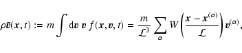
define the Klimontovich density in the one-particle phase space as:
 |
(4b) |
 |
(6b) |
 |
(6c) |
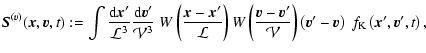
![$\displaystyle %
{\vec S}^{(g)} ({\vec{x}}, {\vec{v}}, t) :=
\int \frac{{\rm d}{...
...ec{g}}({\vec{x}}, t)\right] ~ f_{\rm K} \left({\vec{x}}', {\vec{v}}', t\right).$](/articles/aa/full/2005/29/aa2885-05/img29.gif) |
(6d) |
The field
![]() defined by Eqs. (6b) is the
gravitational mean field associated with the phase-space
density
defined by Eqs. (6b) is the
gravitational mean field associated with the phase-space
density
![]() .
The terms
.
The terms
![]() and
and
![]() represent the dynamical coupling to the degrees of freedom removed
by the smoothing procedure:
represent the dynamical coupling to the degrees of freedom removed
by the smoothing procedure:
![]() accounts for the velocity
dispersion, while
accounts for the velocity
dispersion, while
![]() represents departures from the mean
field gravity on the smoothing scales. Notice that
Eq. (6a) is, like the exact Eq. (4a), a
conservation equation in the one-particle phase space, since the total
number of particles
represents departures from the mean
field gravity on the smoothing scales. Notice that
Eq. (6a) is, like the exact Eq. (4a), a
conservation equation in the one-particle phase space, since the total
number of particles
![]() .
.
Equations (6a,b) do not form a closed system of equations
unless the sources
![]() ,
,
![]() can be
represented or approximated as functionals of
can be
represented or approximated as functionals of
![]() .
The form
and success of the approximation depends in general on the initial
conditions and the choice of the coarsening scales
.
The form
and success of the approximation depends in general on the initial
conditions and the choice of the coarsening scales ![]() ,
,
![]() .
A frequently used approximation in many examples of cosmological
and astrophysical interest consists of neglecting small-scale departures
from the coarse variables,
.
A frequently used approximation in many examples of cosmological
and astrophysical interest consists of neglecting small-scale departures
from the coarse variables,
![]() ,
,
![]() ,
so that Eqs. (6a,b) reduce to the
Vlasov-Poisson system of equations for a smooth
,
so that Eqs. (6a,b) reduce to the
Vlasov-Poisson system of equations for a smooth
![]() (e.g.,
Peebles 1980; Binney & Tremaine 1987).
(e.g.,
Peebles 1980; Binney & Tremaine 1987).
However, to describe the formation of cosmological
structures, the continuous phase-space density
![]() is still
too detailed, since the observables we are interested in
are the large-scale density and velocity fields. A mass density and a
mean fluid velocity can be defined by the velocity moments of
is still
too detailed, since the observables we are interested in
are the large-scale density and velocity fields. A mass density and a
mean fluid velocity can be defined by the velocity moments of
![]() :
:
 |
(7b) |
The evolution equations for these two fields, expressing mass and
momentum conservation, follow immediately from Eqs. (6)
or from Eqs. (1)-(2):
 |
(8b) |
| (8c) |
![\begin{eqnarray*}{\cal P}_{ij} ({\vec{x}}, t) &:= &
m \int {\rm d}{\vec{v}}\Big...
...\vec{x}}, t) \right] S_i^{(v)}({\vec{x}}, {\vec{v}}, t) \Bigr\}
\end{eqnarray*}](/articles/aa/full/2005/29/aa2885-05/img48.gif)
![\begin{displaymath}%
\hspace*{1.3cm} = \frac{m}{{\cal L}^3} \sum_\alpha
W \lef...
...v_j^{(\alpha)} - {\bar v}_i {\bar v}_j ({\vec{x}}, t)\right].
\end{displaymath}](/articles/aa/full/2005/29/aa2885-05/img49.gif) |
(9b) |
The set of hydrodynamic-like Eqs. (8) can be derived through the intermediate step of a kinetic equation, Eq. (6a), or directly from the microscopic particle
dynamics, Eqs. (1). In the latter case, ![]() disappears from the
definitions (7, 9) after
integrating over the velocities, indicating that the precise value of
disappears from the
definitions (7, 9) after
integrating over the velocities, indicating that the precise value of ![]() is unimportant for
Eqs. (8).
is unimportant for
Eqs. (8).
An advantage of the formal derivation through coarse-graining as
presented here is that it makes explicit the smoothing scales ![]() and
and ![]() ,
which are usually implicit in most applications
and not clearly presented. Although these two scales are arbitrary,
their choice is usually dictated by the physics of the problem at hand.
Typically
,
which are usually implicit in most applications
and not clearly presented. Although these two scales are arbitrary,
their choice is usually dictated by the physics of the problem at hand.
Typically
![]() ,
and we know of only one application where
,
and we know of only one application where
![]() :
the numerical codes to solve the Vlasov equation necessarily have a finite resolution in phase-space and
coarse-graining in velocity is a method to treat the
filamentation problem in velocity space induced by this equation
(Klimas 1987). (In other works (e.g. Lynden-Bell 1967; Shu 1978)
phase-space coarsening is invoked but the precise value of
:
the numerical codes to solve the Vlasov equation necessarily have a finite resolution in phase-space and
coarse-graining in velocity is a method to treat the
filamentation problem in velocity space induced by this equation
(Klimas 1987). (In other works (e.g. Lynden-Bell 1967; Shu 1978)
phase-space coarsening is invoked but the precise value of ![]() ,
being irrelevant, is not addressed).
,
being irrelevant, is not addressed).
The spatial scale ![]() is usually chosen in concordance with the
length scale of the phenomena of interest. In the regimes of
validity of the paradigmatic examples of kinetic theory (Boltzmann
equation and Vlasov equation),
is usually chosen in concordance with the
length scale of the phenomena of interest. In the regimes of
validity of the paradigmatic examples of kinetic theory (Boltzmann
equation and Vlasov equation), ![]() is much larger than the mean
interparticle distance
is much larger than the mean
interparticle distance ![]() ,
so that
,
so that
![]() does not resemble the
spiky Klimontovich density
does not resemble the
spiky Klimontovich density
![]() (Spohn 1991,
and refs. therein). The Boltzmann equation for dilute gases with
a short range
(Spohn 1991,
and refs. therein). The Boltzmann equation for dilute gases with
a short range ![]() of interaction
follows from Eq. (6a) when the mean field force
of interaction
follows from Eq. (6a) when the mean field force
![]() is negligible compared to the effect of the term
is negligible compared to the effect of the term
![]() ,
which is dominated by binary "close encounters'' of
uncorrelated particles.
This holds in the scaling limit
,
which is dominated by binary "close encounters'' of
uncorrelated particles.
This holds in the scaling limit
![]() with
with
![]() (dilute limit) and
(dilute limit) and
![]() (continuum
limit), and the mean free path,
(continuum
limit), and the mean free path,
![]() ,
remains finite.
The Vlasov equation describes the dynamical evolution of
,
remains finite.
The Vlasov equation describes the dynamical evolution of
![]() when the interaction is long-ranged and weak. For the gravitational interaction, Eqs. (2), this holds in the
scaling limit
when the interaction is long-ranged and weak. For the gravitational interaction, Eqs. (2), this holds in the
scaling limit
![]() with
with
![]() (finite mass
density) and
(finite mass
density) and
![]() (continuum limit), so that the
particle distribution is statistically homogeneous on scales below
(continuum limit), so that the
particle distribution is statistically homogeneous on scales below ![]() and the mean field
and the mean field
![]() dominates over the effect
of "close encounters'' contained in
dominates over the effect
of "close encounters'' contained in
![]() .
.
Ma & Bertschinger (2004) study the Klimontovich equation
for particles moving in a given stochastic large-scale gravitational field,
intended to be a model of particle evolution
in a galaxy halo environment; after averaging over realizations of the large-scale
gravitational field a new kinetic equation for the ensemble averaged f is obtained
that differs from the Vlasov equation (this ensemble averaging is, in the language of
statistical physics, similar to an average over "disorder'' rather than
an average over "thermal noise'').
For comparison, our Eqs. (6)
describe the evolution of a single realization of a coarse-grained distribution
(note that the mathematical structure of both averaging approaches are similar with
reinterpretation of the window function ![]() as a probability density).
Of course, in addition to coarse-graining one could implement ensemble averaging.
The addition of a noise term as a model of small-scale degrees of freedom involves
interesting physics
(e.g., Berera & Fang 1994; Barbero et al. 1997; Domínguez et al. 1999;
Buchert et al. 1999; Matarrese & Mohayaee 2002; Antonov 2004).
as a probability density).
Of course, in addition to coarse-graining one could implement ensemble averaging.
The addition of a noise term as a model of small-scale degrees of freedom involves
interesting physics
(e.g., Berera & Fang 1994; Barbero et al. 1997; Domínguez et al. 1999;
Buchert et al. 1999; Matarrese & Mohayaee 2002; Antonov 2004).
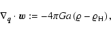
In this section we apply the method of coarse-graining to the
case of structure formation in cosmology by gravitational instability.
In this case it is convenient to introduce "comoving'' Eulerian
coordinates attached to a homogeneous-isotropic
solution (Friedmann-Lemaître backgrounds), characterized by the
expansion factor a(t) (and Hubble's function
![]() ), with
tiny inhomogeneities superimposed as the seeds of structure formation.
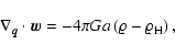
In order to subtract the homogeneous-isotropic motion, one defines
comoving positions
), with
tiny inhomogeneities superimposed as the seeds of structure formation.
In order to subtract the homogeneous-isotropic motion, one defines
comoving positions
![]() ,
peculiar-velocities
,
peculiar-velocities
![]() and gravitational peculiar-accelerations
and gravitational peculiar-accelerations
![]() as follows:
as follows:
where
![]() is the (comoving) coarsening length. This length is in
principle arbitrary, its use being motivated by the features of
cosmological structure formation one is interested in.
In general, one should demand that L will be much larger than the (comoving) mean interparticle
distance, since dark matter discreteness is cosmologically irrelevant.
In the rest of the paper, when we speak about "small/large scales'', we
use L to set the comparison scale.
is the (comoving) coarsening length. This length is in
principle arbitrary, its use being motivated by the features of
cosmological structure formation one is interested in.
In general, one should demand that L will be much larger than the (comoving) mean interparticle
distance, since dark matter discreteness is cosmologically irrelevant.
In the rest of the paper, when we speak about "small/large scales'', we
use L to set the comparison scale.
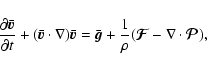
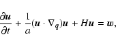
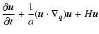
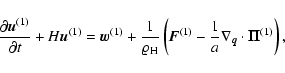
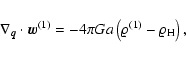
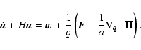
The equations obeyed by these fields can be derived as before. Note that,
in the following we drop the overbar used to distinguish
the microscopic velocities and accelerations from the mean velocities and
mean field strengths; we
always refer to the following equations, so that we no longer need this
distinction (the time-derivative is taken at constant ![]() and L in these equations; see Appendix A for
the relation to Eqs. (8)):
and L in these equations; see Appendix A for
the relation to Eqs. (8)):
 |
(13b) |
 |
(13c) |
 |
(13d) |
![\begin{displaymath}%
\Pi_{ij} ({\vec{q}}, t) := \frac{m}{(a L)^3} \sum_\alpha W ...
...\alpha)} u_j^{(\alpha)} - {u}_i {u}_j ({\vec{q}}, t) \right].
\end{displaymath}](/articles/aa/full/2005/29/aa2885-05/img87.gif) |
(14b) |
In the context of cosmological structure formation one cannot follow this argument, since the notion of thermal equilibrium is not well-defined. We instead discuss three closures:
1. The "dust model'': one assumes that the large-scale dynamics
is dominated by the large-scale forces and neglects the coupling to
the small scales altogether: one sets
![]() ,
,
![]() in Eqs. (13), and obtains the Euler-Newton system for
the peculiar-fields:
in Eqs. (13), and obtains the Euler-Newton system for
the peculiar-fields:
 |
(15b) |
 |
(15c) |
 |
(15d) |
The "dust model'' was originally applied to the "top-down scenario'' of structure formation, e.g., "Hot Dark Matter cosmogony'', in which large-scale density inhomogeneities grow while the small scales remain homogeneous. The model, however, turned out to be a relatively good description also for the "bottom-up scenario'', e.g., "Cold Dark Matter cosmogony'' (Pauls & Melott 1995), in which the small scales are always strongly inhomogeneous. Strictly speaking, the "dust model'' is not properly defined if there is too much initial small-scale power, because of the emergence of singularities at arbitrarily short times, so that a small-scale cutoff is required (this becomes manifest in formal perturbative expansions too, Valageas 2002; Bernardeau et al. 2002). Our derivation of the "dust model'' clearly demonstrates that the smoothing length L is indeed a defining ingredient of the model. However, this fact has not been properly emphasized in the literature - the smoothing length is likely irrelevant in the "top-down scenario'', where the initial conditions have a built-in length of smoothness (free-flight scale of the dark matter particles), but this is not so in a "bottom-up scenario'': in this latter case, it was found that a much better agreement with N-body simulations is achieved if the initial conditions are first smoothed, e.g., the "Truncated Zel'dovich Approximation'' (Coles et al. 1993).
The "dust model'' correctly describes many features of the formation of
structure by gravitational instability. It has also an important
shortcoming, which is the focus of the present work, namely that it
generates caustics, i.e., density singularities, as well as multi-streaming regions (shell-crossing), where the velocity
field is multi-valued. This points to a breakdown of the
approximation, so that the term
![]() in
Eq. (13b) is no longer negligible.
In the present work we address
two approximations beyond the "dust model'' in which this term is
modelled as a function of
in
Eq. (13b) is no longer negligible.
In the present work we address
two approximations beyond the "dust model'' in which this term is
modelled as a function of ![]() and
and ![]() .
.
2. The Euler-Jeans-Newton ("EJN'') model: motivated by
hydrodynamics and the theory of stellar systems, we have the
following phenomenological closure: the corrections to mean field gravity are
neglected, and the velocity dispersion
is approximated by an isotropic tensor field which, in addition, is commonly
modelled as a function of the local density:
Given the phenomenological character of the
approximation (16), one can think of the relationship
![]() as "templates'' modeling the overall effect of both velocity dispersion
and departure from mean field gravity as long as the mathematical
analysis of Eqs. (17) is involved. The only exact constraint
required by this interpretation is that
as "templates'' modeling the overall effect of both velocity dispersion
and departure from mean field gravity as long as the mathematical
analysis of Eqs. (17) is involved. The only exact constraint
required by this interpretation is that ![]() can be written as the
divergence of a stress tensor. This is the case in the other
closure ansatz to be discussed (see Eq. (20)).
can be written as the
divergence of a stress tensor. This is the case in the other
closure ansatz to be discussed (see Eq. (20)).
Inserting the ansatz for Fi and ![]() into
Eq. (13b), one gets (
into
Eq. (13b), one gets (
![]() is the
Laplacian operator in the variable
is the
Laplacian operator in the variable ![]() ):
):
 |
= |  |
|
| = |  |
(17b) |
 |
(17c) |
 |
(17d) |
The case of isotropic stresses formally covers the hydrodynamics of a perfect fluid or, as common in studies of stellar systems, polytropic models. However, there is no compelling reason for isotropic stresses in collisionless systems before the onset of virialization. Even "virialized'' systems will in general maintain an anisotropic component. At the moment, we consider the isotropy assumption as a good working hypothesis to understand the role of interaction between multi-stream forces and self-gravity: the velocity dispersion ellipsoid is approximated by a sphere. (Interesting considerations of the influence of the anisotropic part have been reported by Maartens et al. 1999; see also Barrow & Maartens 1999.)
3. The Small-Size Expansion ("SSE''): this is a method proposed
by Domínguez (2000, 2002) to formalize the notion that
the coupling to the small scales is in some sense weak.
One argues that the corrections Fi and
![]() are determined
mainly by the largest scales contributing to them, i.e., those close
to L. For instance, in the bottom-up scenario,
the large-scale dynamics is sensitive mainly to the
motion of the most recently formed clusters as a whole, and not so much to
their internal structural details due to the trapped particles, so that one takes
are determined
mainly by the largest scales contributing to them, i.e., those close
to L. For instance, in the bottom-up scenario,
the large-scale dynamics is sensitive mainly to the
motion of the most recently formed clusters as a whole, and not so much to
their internal structural details due to the trapped particles, so that one takes ![]() typical size of these clusters (which play the role of effective
particles of size
typical size of these clusters (which play the role of effective
particles of size ![]() L).
The mathematical implementation of this idea leads to a formal
expansion of Fi and
L).
The mathematical implementation of this idea leads to a formal
expansion of Fi and ![]() in powers of the smoothing
length
in powers of the smoothing
length![]() L (see
Appendix B for an outline of the derivation):
L (see
Appendix B for an outline of the derivation):
 |
(19b) |
| |
 |
||
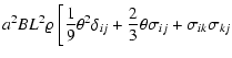
![$\displaystyle + \frac{1}{4} \left(\omega^2 \delta_{ij} - \omega_i \omega_j\right) \biggr] + {\cal O}\left(L^4\right).$](/articles/aa/full/2005/29/aa2885-05/img125.gif) |
(22) |
| |
+ | ||
![$\displaystyle + \frac{B L^2}{\varrho} \left\{ \left(\nabla_{\vec{q}}\varrho \cd...
...ot \left[\varrho (\partial_k {\vec{u}}) (\partial_k {\vec{u}})\right] \right\},$](/articles/aa/full/2005/29/aa2885-05/img130.gif) |
(23b) |
|
(23c) |
|
(23d) |
The closure assumption (19b) for the velocity
dispersion has been also used to model the influence of
subresolution degrees of freedom of the velocity field in
"Large-Eddy Simulations'' of turbulent flow (Pope 2000). It has
been termed the "gradient model'' (see, e.g., Vreman et al. 1997) and it
was introduced as part of the "Clark model'' (Clark et al. 1979) (a
model which includes an extra additive term in the expression
for ![]() ).
).
Both the "EJN'' and the "SSE'' models provide an extension of the "dust model''
with the potential to improve on it by preventing the formation of
singularities. The "EJN model'' relies on a phenomenological assumption
concerning the kinetic stress ![]() ,
but has the advantage that
the resulting equations are well established. In favor of the "SSE''
model is the fact that the corrections to "dust'' can be obtained
systematically beyond phenomenology, but the mathematical and physical
status of the resulting equations is little explored yet.
,
but has the advantage that
the resulting equations are well established. In favor of the "SSE''
model is the fact that the corrections to "dust'' can be obtained
systematically beyond phenomenology, but the mathematical and physical
status of the resulting equations is little explored yet.
In this subsection we get a first picture of the effect of the
corrections to the "dust model''.
In the "adhesion model'' (Gurbatov et al. 1989), the evolution
of "dust'' is modelled with Zel'dovich's approximation (Zel'dovich
1970, 1973), a powerful and mathematically manageable description of
the exact evolution (first-order Lagrangian perturbation solution,
see Sect. 5.1). Accordingly, one assumes in
Eq. (15b) the proportionality of peculiar-velocity and
-acceleration fields (cf. Peebles 1980; Buchert 1989, 1992;
Bildhauer & Buchert 1991; Kofman 1991; Buchert 1993b; Vergassola et al. 1994):
![\begin{displaymath}\frac{1}{\varrho} \left[ F_i - \frac{1}{a} \Pi_{ij,j} \right]...
...t(\nabla_{\vec{q}}\cdot {\vec{u}}\right) \Delta_{\vec{q}}u_i.
\end{displaymath}](/articles/aa/full/2005/29/aa2885-05/img144.gif)
Equation (26) resembles the well-known key equation of the
original "adhesion approximation'' (Gurbatov et al. 1989), to
which it reduces when ![]() = constant
= constant
![]() .
For constant
.
For constant ![]() it can be solved analytically for curl-free flows (Hopf-Cole transformation of the 3D Burgers' equation); this solution shows that the
singularities predicted by the "Zel'dovich approximation'',
Eq. (25), are indeed regularized by the
it can be solved analytically for curl-free flows (Hopf-Cole transformation of the 3D Burgers' equation); this solution shows that the
singularities predicted by the "Zel'dovich approximation'',
Eq. (25), are indeed regularized by the ![]() -term (see,
e.g., Vergassola et al. 1994); for an interesting application of Burgers' equation and further insight see also the model of Jones (1996) for a two-component system.
In the more general cases of a density-dependent GM coefficient, no
analytical solution was found. Nevertheless, the application of
boundary-layer theory (Domínguez 2000) shows that density
singularities are still regularized (provided
-term (see,
e.g., Vergassola et al. 1994); for an interesting application of Burgers' equation and further insight see also the model of Jones (1996) for a two-component system.
In the more general cases of a density-dependent GM coefficient, no
analytical solution was found. Nevertheless, the application of
boundary-layer theory (Domínguez 2000) shows that density
singularities are still regularized (provided
![]() with
with ![]() in the case of the "EJN model'', so that pressure can oppose gravity successfully). The solutions for the velocity and density fields are qualitatively
identical to those of the original "adhesion model'', developing into a
shock structure of infinite density in the limit
in the case of the "EJN model'', so that pressure can oppose gravity successfully). The solutions for the velocity and density fields are qualitatively
identical to those of the original "adhesion model'', developing into a
shock structure of infinite density in the limit
![]() .
.
This derivation of the "adhesion approximation'' offers insight into
the physics involved. The ![]() -term, which was phenomenologically
motivated by analogy with viscosity, is not related to a truly
dissipative process.
From a mathematical point of view, the starting point ("EJN model'' (17) or "SSE model'' (23)), the approximations,
and the final Eq. (26) are formally time-reversible,
i.e., invariant under the transformation
-term, which was phenomenologically
motivated by analogy with viscosity, is not related to a truly
dissipative process.
From a mathematical point of view, the starting point ("EJN model'' (17) or "SSE model'' (23)), the approximations,
and the final Eq. (26) are formally time-reversible,
i.e., invariant under the transformation
![]() ,
,
![]() .
The correction to "dust'' can transform mean kinetic energy (
.
The correction to "dust'' can transform mean kinetic energy (![]()
![]() )
into internal kinetic energy (
)
into internal kinetic energy (![]()
![]() )
and conversely (also into internal gravitational potential energy via Fi, but, as we have shown, the "SSE model'' predicts this
contribution to be subdominant near density singularities in the
present approximation). The tendency to compression in collapsing
regions favors the correction to behave as a drain of mean kinetic
energy, mimicking viscous dissipation; it is easy to check that the
correction supplies energy in expanding regions
(see Sect. 6.4), whose expansion is thus accelerated. This mechanism seems to be universal: this is the reason that "adhesiveness'' arises in the two different
models we study, "EJN'' and "SSE'', and that it can be modelled in a
qualitatively correct manner by the simplified "adhesion model''
)
and conversely (also into internal gravitational potential energy via Fi, but, as we have shown, the "SSE model'' predicts this
contribution to be subdominant near density singularities in the
present approximation). The tendency to compression in collapsing
regions favors the correction to behave as a drain of mean kinetic
energy, mimicking viscous dissipation; it is easy to check that the
correction supplies energy in expanding regions
(see Sect. 6.4), whose expansion is thus accelerated. This mechanism seems to be universal: this is the reason that "adhesiveness'' arises in the two different
models we study, "EJN'' and "SSE'', and that it can be modelled in a
qualitatively correct manner by the simplified "adhesion model'' ![]() =
constant. The GM coefficient depends on time and on density, and this
leads to differences between models concerning the inner structure of
the regularized density singularities. A
density independent GM coefficient (as in the original "adhesion
approximation'') is obtained with the imposed relationship
=
constant. The GM coefficient depends on time and on density, and this
leads to differences between models concerning the inner structure of
the regularized density singularities. A
density independent GM coefficient (as in the original "adhesion
approximation'') is obtained with the imposed relationship
![]() corresponding to the naive application of the virial
condition, while the "EJN'' and the "SSE'' models coincide when
corresponding to the naive application of the virial
condition, while the "EJN'' and the "SSE'' models coincide when
![]() .
.
Summarizing, to derive Eq. (26) one makes two important assumptions:
While relaxing (1) implies construction of sophisticated non-perturbative
approximations (since only then can we expect to substantially improve on the
performance of Lagrangian perturbation schemes, optimized to match N-body
simulations for any kind of dark matter),
assumption (2) appears more like an unnecessary simplification. It is crucial
for the derivation of equations similar to the
key equation of the standard "adhesion approximation'', but
it must be relaxed if one intends to improve over the "adhesion model''
in order to describe the subsequent dynamical evolution inside the
collapsing structures.
Assumption (2) may be rephrased by saying that the
evolution is dominated by convection,
![]() ,
over "viscosity'',
,
over "viscosity'',
![]() - in
the hydrodynamic jargon, this is the limit "Reynolds number
- in
the hydrodynamic jargon, this is the limit "Reynolds number
![]() ''. Relaxing this assumption, i.e. finite
Reynolds number, means taking account of the back-reaction of the
correction to "dust'' on the trajectories of fluid elements away from
singularities too. In general, this will also imply corrections to the
parallelism of
''. Relaxing this assumption, i.e. finite
Reynolds number, means taking account of the back-reaction of the
correction to "dust'' on the trajectories of fluid elements away from
singularities too. In general, this will also imply corrections to the
parallelism of ![]() and
and ![]() as well as those due to the exact "dust''
evolution (see, e.g., Eq. (35)).
as well as those due to the exact "dust''
evolution (see, e.g., Eq. (35)).
Menci (2002) has studied the correction to the original
"adhesion approximation'' when assumption (1) is relaxed. The starting
point is the set of Eqs. (13) with the correction to
"dust'' already modelled as
![]() ,
,
![]() constant
constant ![]() .
The correction to parallelism,
.
The correction to parallelism,
![]() ,
is estimated perturbatively in the limit of small velocities or times (the initial condition is taken to satisfy parallelism) - the procedure employed
by Menci is not an expansion in the "viscosity''
,
is estimated perturbatively in the limit of small velocities or times (the initial condition is taken to satisfy parallelism) - the procedure employed
by Menci is not an expansion in the "viscosity'' ![]() ,
although it might formally appear so. The results agree somewhat
better with N-body simulations concerning the details of the forming
structures at small scales.
,
although it might formally appear so. The results agree somewhat
better with N-body simulations concerning the details of the forming
structures at small scales.
The solution to the "adhesion model'', Eq. (26a) with
constant ![]() ,
cannot be computed as a regular expansion in
,
cannot be computed as a regular expansion in ![]() ,
because the naive
zeroth-order term, given by Eq. (25), is undefined after shell-crossing.
The exact analytical solution to this model demonstrates
that the limit
,
because the naive
zeroth-order term, given by Eq. (25), is undefined after shell-crossing.
The exact analytical solution to this model demonstrates
that the limit
![]() yields a weak solution of
Eq. (25), exhibiting discontinuities in
yields a weak solution of
Eq. (25), exhibiting discontinuities in ![]() .
In the pedagogical review
by Frisch & Bec (2001) it is illustrated how much the Lagrangian solution of
a "multi-streamed dust model'' differs from the Lagrangian solution to
the "adhesion model'' after shell-crossing. In particular, it is
explained how the emergence of multi-streaming cannot be captured by a
Taylor expansion in the time variable of the solution to
Eq. (25). As a matter of fact, the corresponding
perturbative expansion of the solution to the Vlasov-Poisson system
is identical to the one of the "dust model'' when the initial condition
is exactly single-streamed
(Valageas 2001)
.
In the pedagogical review
by Frisch & Bec (2001) it is illustrated how much the Lagrangian solution of
a "multi-streamed dust model'' differs from the Lagrangian solution to
the "adhesion model'' after shell-crossing. In particular, it is
explained how the emergence of multi-streaming cannot be captured by a
Taylor expansion in the time variable of the solution to
Eq. (25). As a matter of fact, the corresponding
perturbative expansion of the solution to the Vlasov-Poisson system
is identical to the one of the "dust model'' when the initial condition
is exactly single-streamed
(Valageas 2001)![]() . This
problem can be overridden if a small amount of multi-streaming is allowed in the initial conditions, e.g. in the form of velocity dispersion.
. This
problem can be overridden if a small amount of multi-streaming is allowed in the initial conditions, e.g. in the form of velocity dispersion.
Ribeiro & Peixoto de Faria (2005) also attempted to provide a physical
motivation for the "adhesion model'': starting from the
velocity potential ![]() (with
(with
![]() ), it
is assumed that the complex variable
), it
is assumed that the complex variable
![]() obeys a Schrödinger equation, where
obeys a Schrödinger equation, where ![]() is
a constant with the appropriate dimension. From this assumption, it
is found that
is
a constant with the appropriate dimension. From this assumption, it
is found that ![]() satisfies Eq. (13b) with
a correction to "dust'' that can be written as a functional of the density.
It is not obvious that with this correction term one can recover the "adhesion
model'': it cannot be brought into a simple form
satisfies Eq. (13b) with
a correction to "dust'' that can be written as a functional of the density.
It is not obvious that with this correction term one can recover the "adhesion
model'': it cannot be brought into a simple form
![]() after using the parallelism approximation, and the reasoning
offered by the authors is wrong from the outset because their
Eq. (31) is algebraically false.
after using the parallelism approximation, and the reasoning
offered by the authors is wrong from the outset because their
Eq. (31) is algebraically false.
In the following sections we study the "EJN'' and the "SSE'' models beyond
assumptions (1, 2). First, we consider the standard Eulerian and Lagrangian perturbative
expansions, both closely related to the expansion in time just mentioned.
One of the key points in the derivation of the "adhesion
model'' is the parallelism relation between ![]() and
and ![]() ,
Eq. (24). This relation holds at the (Eulerian as
well as Lagrangian) linear order of the "dust model''.
Application of the perturbative techniques to the "EJN'' and "SSE'' models
will show how this relation is modified by the correction to "dust''.
Later we consider non-perturbative approaches: this is a
mathematically difficult task, and we are only able to collect some
results and provide some hints for future work.
,
Eq. (24). This relation holds at the (Eulerian as
well as Lagrangian) linear order of the "dust model''.
Application of the perturbative techniques to the "EJN'' and "SSE'' models
will show how this relation is modified by the correction to "dust''.
Later we consider non-perturbative approaches: this is a
mathematically difficult task, and we are only able to collect some
results and provide some hints for future work.
The expansion parameter of the Eulerian perturbative expansion is the
amplitude of the departures of the initial conditions from homogeneity.
Formally, one writes:
![\begin{displaymath}%
\sigma^2 (t) := \frac{\left\langle \left[\varrho({\vec{0}},...
...{\rm H}(t)\right]^2 \right\rangle}{\varrho^2_{\rm H} (t)}\cdot
\end{displaymath}](/articles/aa/full/2005/29/aa2885-05/img173.gif) |
(30) |
To this order, one obtains the following equations:
 |
(31b) |
 |
(31c) |
 |
(31d) |
The "EJN model'' provides a correction to the parallelism relation
already at the linear order. Following Buchert et al. (1999)![]() , the solution to Eq. (34) and the
departure from parallelism can be computed as a series in powers of
, the solution to Eq. (34) and the
departure from parallelism can be computed as a series in powers of ![]() (unlike in the fully non-linear problem, the limit
(unlike in the fully non-linear problem, the limit
![]() in Eq. (34) is regular). Asymptotically in time, we may write (
in Eq. (34) is regular). Asymptotically in time, we may write (
![]() is a dimensionless
time-dependent coefficient):
is a dimensionless
time-dependent coefficient):
The Eulerian perturbative expansion beyond the linear order has been
intensively studied for the "dust model'' in recent years (see,
e.g., Bernardeau et al. 2002 and references therein). The predictions of the
"SSE model'' differ from those of the "dust model'' at non-linear orders.
An important difference concerns the vorticity. With full generality
(i.e., to all orders of the perturbative expansion), one can easily show from
Eq. (13b)
by application of the vector identity
![]() that (here, a comma denotes partial
derivative with respect to comoving Eulerian coordinates)
that (here, a comma denotes partial
derivative with respect to comoving Eulerian coordinates)
![\begin{displaymath}%
\frac{\partial \omega_i^{(2)}}{\partial t} + 2H \omega_i^{(...
...{1}{a} \left(u_{m,l}^{(1)} u_{k,l}^{(1)}\right)_{,jm} \right].
\end{displaymath}](/articles/aa/full/2005/29/aa2885-05/img211.gif) |
(38) |
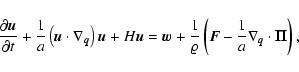
To perform the Lagrangian perturbative expansion, we have to transform the
equations with respect to Lagrangian coordinates and follow the field
quantities along comoving trajectories of the fluid elements:
In view of later considerations, for the application of the Lagrangian methods we take an
unconventional route and first rewrite Eqs. (13) as
follows. We obtain an evolution equation for the peculiar-gravitational field ![]() by eliminating the density in Eq. (13a) with the help of Eq. (13c).
By formally integrating the divergence one gets (Buchert 1989):
by eliminating the density in Eq. (13a) with the help of Eq. (13c).
By formally integrating the divergence one gets (Buchert 1989):
| |
= | ||
| = | (40b) |
 |
(40c) |
For the "dust model'' the system of Eqs. (40a-c) has been studied thoroughly in (Buchert
1989). There, the currently used notion of the weakly non-linear
regime has been defined as "Lagrangian linearization''.
The comoving trajectory field ![]() of Zel'dovich's approximation
(Zel'dovich 1970, 1973) can be understood as a subclass of the
linear solutions in Lagrangian space (Buchert 1989, 1992). For an Einstein-de Sitter cosmology
with initial peculiar-velocity
of Zel'dovich's approximation
(Zel'dovich 1970, 1973) can be understood as a subclass of the
linear solutions in Lagrangian space (Buchert 1989, 1992). For an Einstein-de Sitter cosmology
with initial peculiar-velocity
![]() ,
the subclass
corresponding to Zel'dovich's model is
,
the subclass
corresponding to Zel'dovich's model is
![]() ,
where
b(t)=a(t) here. For all background cosmologies including "curvature'' and a cosmological
constant Zel'dovich's approximation is given in (Bildhauer et al. 1992; for
the flat models with cosmological constant, see also the supplement by
Chernin et al. 2003).
,
where
b(t)=a(t) here. For all background cosmologies including "curvature'' and a cosmological
constant Zel'dovich's approximation is given in (Bildhauer et al. 1992; for
the flat models with cosmological constant, see also the supplement by
Chernin et al. 2003).
This well-known result can be easily obtained from the general
system of Eqs. (40a-c) by the following reasoning:
in the Lagrangian picture the Eulerian dynamical variables
![]() and
and
![]() are replaced by the single dynamical variable
are replaced by the single dynamical variable
![]() .
Lagrangian linearization means that the
equations have to be linearized with respect to
.
Lagrangian linearization means that the
equations have to be linearized with respect to ![]() .
Equations (39) and (40c) (without corrections to "dust'') express the fields
.
Equations (39) and (40c) (without corrections to "dust'') express the fields ![]() and
and ![]() as linear functions of
as linear functions of ![]() .
It follows that Eqs. (40a,b) have to be linearized in the fields
.
It follows that Eqs. (40a,b) have to be linearized in the fields ![]() and
and ![]() .
For simplicity we restrict the initial conditions to
irrotational flow, so that the velocity remains irrotational through
the "dust'' evolution, Eq. (37). Then, Eq. (40b) implies, upon linearization,
.
For simplicity we restrict the initial conditions to
irrotational flow, so that the velocity remains irrotational through
the "dust'' evolution, Eq. (37). Then, Eq. (40b) implies, upon linearization,
![]() .
From Eq. (40a) we can therefore immediately drop the manifestly
non-linear terms in the residual vector field
.
From Eq. (40a) we can therefore immediately drop the manifestly
non-linear terms in the residual vector field
![]() .
Introducing the longitudinal and transversal parts of
.
Introducing the longitudinal and transversal parts of ![]() and
and ![]() with respect to Lagrangian coordinates, e.g.,
with respect to Lagrangian coordinates, e.g.,
![]() ,
,
![]() ,
where
,
where
![]() denotes the nabla operator with respect to Lagrangian coordinates, the
remaining equations for "dust'' read:
denotes the nabla operator with respect to Lagrangian coordinates, the
remaining equations for "dust'' read:
In the regime when the "dust model'' predicts multi-streaming, the
corrections to "dust'' become relevant.
We look for the Lagrangian linear form by also dropping the
residual vector field
![]() (since initial irrotationality is
preserved to linear order by the evolution in both the "EJN'' and the
"SSE model'').
The "SSE'' correction to "dust'' is also non-linear, Eq. (23b), so that this
model does not differ from the "dust model'' to linear order.
For the "EJN model'', Eq. (17b), however,
we have to linearize additionally the
(Eulerian) Laplacian together with the GM coefficient
along the comoving trajectory field. Using
transformation tools developed by Adler & Buchert (1999, Appendix A)
we find (for isotropic
(since initial irrotationality is
preserved to linear order by the evolution in both the "EJN'' and the
"SSE model'').
The "SSE'' correction to "dust'' is also non-linear, Eq. (23b), so that this
model does not differ from the "dust model'' to linear order.
For the "EJN model'', Eq. (17b), however,
we have to linearize additionally the
(Eulerian) Laplacian together with the GM coefficient
along the comoving trajectory field. Using
transformation tools developed by Adler & Buchert (1999, Appendix A)
we find (for isotropic
![]() ):
):
Evidently, the adhesive term consists of a Lagrangian Laplacian and,
therefore, it involves, in addition to the convective non-linearities
hidden in the overdot, non-linearities in Eulerian space
when mapping it back
using the inverse solution of the mapping
![]() .
.
In general, parallelism of peculiar-velocity and
-acceleration is violated. By computing the time derivative of
the difference
![]() with Eqs. (45), one can show
that in general it does not decay to zero asymptotically for large
times. The correction is proportional to
with Eqs. (45), one can show
that in general it does not decay to zero asymptotically for large
times. The correction is proportional to
![]() to
lowest order in
to
lowest order in ![]() .
This correction is similar to the one found in
the Eulerian linear approximation, Eq. (35), but in
terms of the Lagrangian gradients.
.
This correction is similar to the one found in
the Eulerian linear approximation, Eq. (35), but in
terms of the Lagrangian gradients.
The Lagrangian perturbation scheme including pressure (Adler & Buchert 1999) has been pushed to second order (Morita & Tatekawa 2001; Tatekawa e al. 2002) and recently to third order (Tatekawa 2005). Results on cross-correlation statistics with N-body simulations (Tatekawa 2004a) and a comparison of the corresponding density fluctuations with results of hydrodynamical simulations (Tatekawa 2004b) has demonstrated that multi-stream forces tend to be underestimated by Lagrangian perturbative models. In the next section we shall investigate why this happens.
Following a systematic perturbative approach we could provide models for adhesive gravitational clustering in the weakly non-linear regime. This has allowed us also to relax the parallelism assumption (24) that was a necessary ingredient of the standard "adhesion model'' but, as we have shown, is not expected to hold in the multi-streamed regime.
Finding an extension into the non-perturbative (both Eulerian and Lagrangian) regimes is an involved mathematical task. Notwithstanding, it should be attempted in view of the fact that even the Lagrangian perturbation approach falls short of capturing the action of multi-stream forces, since a genuine property of adhesive models in the simplest cases involves an Eulerian Laplacian. Thus, we expect the best approximations to be of hybrid Lagrangian/Eulerian type like the standard "adhesion model'', meaning a non-linear equation both in Eulerian space (due to the convective non-linearities) as well as in Lagrangian space (due to the Eulerian gradients in the forcing).
An exact equation for the comoving deviations of the trajectory field,
![]() defined by Eq. (39), can be obtained from
Eqs. (40): formal integration of Eq. (40a) yields
defined by Eq. (39), can be obtained from
Eqs. (40): formal integration of Eq. (40a) yields
As a further illustration of the general case we write down the corresponding equation
for the density. For this purpose we introduce the contrast density field
![]() ,
,
![]() ,
which is
more adapted to the non-linear situation than the conventional density
contrast
,
which is
more adapted to the non-linear situation than the conventional density
contrast
![]() (for the "dust'' case see:
Buchert 1989 Eq. (7)ff, 1992 Eq. (31)ff, and 1996 Eq. (25)ff
(with a different sign convention for
(for the "dust'' case see:
Buchert 1989 Eq. (7)ff, 1992 Eq. (31)ff, and 1996 Eq. (25)ff
(with a different sign convention for ![]() )).
The exact evolution equation for this variable can be obtained
from Eqs. (13a,b):
)).
The exact evolution equation for this variable can be obtained
from Eqs. (13a,b):
The problem is simplified if one considers particular
geometric settings with high symmetry. Although this leads to
not fully realistic models, it can provide hints of the mathematical
and physical properties of the models in the non-perturbative regime.
Plane-symmetric models provide an
excellent test case for numerical simulations of multi-stream systems concerning a variety of
properties including spatial scaling
(e.g. Doroshkevich et al. 1980; Gouda & Nakamura 1988, 1989; Yano & Gouda 1998; Fanelli & Aurell 2002; Aurell et al. 2003; Yano et al. 2003; the assumption of
spherical symmetry plays a complementary role, e.g. Padmanabhan 1996.)
In such configurations, the fields vary spatially along a single direction, and so
render the Lagrangian approach
particularly suitable for an extension into the non-perturbative
regime. Plane-symmetric models simplify the problem enormously, since
the residual term
![]() vanishes, and the "dust'' evolution remains in the
Lagrangian linear regime at all times (implying in
particular that the parallelism relation (24) - stating a
spatially constant factor of proportionality - holds asymptotically at large times).
vanishes, and the "dust'' evolution remains in the
Lagrangian linear regime at all times (implying in
particular that the parallelism relation (24) - stating a
spatially constant factor of proportionality - holds asymptotically at large times).
In a plane-symmetric configuration, the fields vary only along a
single direction, say i=1. Equations (46), (47), (49), (51)
then are simplified to (we hereafter drop the index i=1):
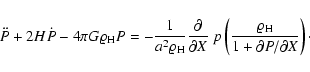 |
(53b) |
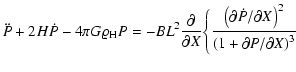 |
|||
![$\displaystyle + 4 \pi G \varrho_{\rm H} \left[ \displaystyle\frac{1}{2 \left(1+...
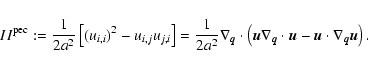
...right)^2} - \displaystyle\frac{1}{1+\partial P/\partial X} \right] \Bigg\}\cdot$](/articles/aa/full/2005/29/aa2885-05/img285.gif) |
(53c) |
Equations (53) should allow one to explore the role of the corrections
to "dust'' beyond the assumptions employed in Sect. 3.1, in
particular, the back-reaction on the "dust'' trajectories by the
correction terms. It should be noted that Eqs. (53)
are of second order in time, in contrast to the generalized
"adhesion model'', Eq. (26a) - the relevance of this fact concerning
the formation of singularities is discussed in Sect. 6.4. In
this connection Eqs. (53b,c) have features of a
quasilinear hyperbolic ("wave'') equation, while Eq. (26a) is a quasilinear parabolic
("diffusion'') equation. Götz (1988) considered the "EJN model'' with the
"isothermal'' relationship
![]() in the absence of
background cosmological expansion (
in the absence of
background cosmological expansion (
![]() ),
and he was able to show that it can be mapped exactly to the Sine-Gordon
equation, which is known to admit soliton solutions.
),
and he was able to show that it can be mapped exactly to the Sine-Gordon
equation, which is known to admit soliton solutions.
Fanelli & Aurell (2002) numerically studied the one-dimensional
Vlasov-Poisson system (see Sect. 2), in particular the
time-dependence of a collapsing isolated perturbation. Fanelli &
Aurell tried to interpret the numerical findings in the framework of
the simplified "EJN model'' (26) with a polytropic
relationship for the pressure,
![]() .
A
simple scaling argument led them to the value
.
A
simple scaling argument led them to the value
![]() (the
original "adhesion model'' corresponding to
(the
original "adhesion model'' corresponding to ![]() ). This
conclusion is, however, questionable because boundary-layer theory
cannot be applied to Eqs. (26) when
). This
conclusion is, however, questionable because boundary-layer theory
cannot be applied to Eqs. (26) when ![]() .
A more
general analysis (Domínguez, unpublished) shows that a
shock can form in this case only when the initial velocity is smaller
than the maximum velocity, and this maximum velocity vanishes in the
limit
.
A more
general analysis (Domínguez, unpublished) shows that a
shock can form in this case only when the initial velocity is smaller
than the maximum velocity, and this maximum velocity vanishes in the
limit
![]() .
That is, when
.
That is, when ![]() ,
the adhesive
term is too weak to prevent singularities for arbitrary initial
velocities. Thus, it might be the case that Eqs. (26)
cannot describe even qualitatively the numerical experiment by
Fanelli & Aurell.
,
the adhesive
term is too weak to prevent singularities for arbitrary initial
velocities. Thus, it might be the case that Eqs. (26)
cannot describe even qualitatively the numerical experiment by
Fanelli & Aurell.
As remarked, one of the difficulties with the exact Eq. (47) is the nonlocal nature introduced by
![]() .
A possible approximation consists therefore in setting
.
A possible approximation consists therefore in setting
![]() ,
so that Eq. (47) simplifies to
,
so that Eq. (47) simplifies to
One can view the approximation
![]() in the same spirit
as the parallelism assumption (24): one gets rid of the
problem of nonlocality by approximating the exact peculiar-gravitational field by
a relationship which holds in the (both
Eulerian and Lagrangian) linear regime of the "dust model'' as well as
exactly in the plane-symmetric configuration:
in the same spirit
as the parallelism assumption (24): one gets rid of the
problem of nonlocality by approximating the exact peculiar-gravitational field by
a relationship which holds in the (both
Eulerian and Lagrangian) linear regime of the "dust model'' as well as
exactly in the plane-symmetric configuration:
To get a glimpse of the mathematical difficulties posed by
Eq. (54), we particularize it to the "EJN model'' of ![]() and
and
![]() ,
Eq. (16). The right-hand-side can be
written, in analogy with Eq. (17b), as:
,
Eq. (16). The right-hand-side can be
written, in analogy with Eq. (17b), as:
In conclusion, we propose the approximation (55) as a first extrapolation into the non-perturbative regime of the Eulerian and Lagrangian linear approximations without resort to the constraining assumption of parallelism. It should be viewed as a simplification of the exact Eqs. (13) in the sense that the approximation yields a local equation, which should facilitate the theoretical analysis. An attempt to solve the approximate equation could be successful, but lies beyond the scope of the present work.
A point one would like to be able to prove rigorously beyond the
argument offered in Sect. 3.1 is whether the "EJN and SSE models'' do indeed prevent the formation of singularities given initial conditions of cosmological relevance.
The absence of singularities when initially smooth data are propagated by the
Vlasov-Poisson system has been proved mathematically
(Lions & Perthame 1991; Schaeffer 1991; Pfaffelmoser 1992; Rein & Rendall 1994). The original "adhesion model'' reduces to the 3D Burgers' equation
(Eq. (26) with constant ![]() ), which has the unusual
property of being solvable analytically. From there, one can demonstrate
that no singularity arises for any sufficiently smooth initial
conditions (see, e.g., Frisch & Bec 2001).
For other models this is a very difficult question (e.g.,
it is still an open problem for the 3-dimensional incompressible
Navier-Stokes equations (Frisch 1995, Sect. 9.3)), and here we can only
provide some general remarks.
), which has the unusual
property of being solvable analytically. From there, one can demonstrate
that no singularity arises for any sufficiently smooth initial
conditions (see, e.g., Frisch & Bec 2001).
For other models this is a very difficult question (e.g.,
it is still an open problem for the 3-dimensional incompressible
Navier-Stokes equations (Frisch 1995, Sect. 9.3)), and here we can only
provide some general remarks.
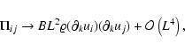
Starting from Eqs. (13), (21), one can derive the
following evolution equations for the density ![]() and the
peculiar-expansion rate
and the
peculiar-expansion rate ![]() :
:
 |
(58b) |
The continuity Eq. (58a) can be integrated in
Lagrangian coordinates:
For the "EJN model'', the correction to "dust'' reads
![]() ,
where p is modelled as a
density-dependent pressure, so that Eqs. (17) have the
structure of the equations of inviscid fluid dynamics. In the absence
of self-gravity, it is known that the solution becomes
non-differentiable for a generic class of smooth initial conditions,
so that the Lagrangian-to-Eulerian map
,
where p is modelled as a
density-dependent pressure, so that Eqs. (17) have the
structure of the equations of inviscid fluid dynamics. In the absence
of self-gravity, it is known that the solution becomes
non-differentiable for a generic class of smooth initial conditions,
so that the Lagrangian-to-Eulerian map
![]() ceases to be
defined. The map can remain uni-valued if we allow for shocks
(moving discontinuities in the fields): this is called a weak
solution, and they have to be understood as solutions of the
differential Eqs. (17) with an additional viscous term
ceases to be
defined. The map can remain uni-valued if we allow for shocks
(moving discontinuities in the fields): this is called a weak
solution, and they have to be understood as solutions of the
differential Eqs. (17) with an additional viscous term
![]() in the limit
in the limit
![]() ,
in the same way as we
discussed for the adhesion model
,
in the same way as we
discussed for the adhesion model![]() . The presence of
self-gravity is not expected to alter this conclusion; the question
is rather whether the initial conditions of cosmological interest
belong to the class of initial conditions inducing shock formation.
The reason for the emergence of shocks can be ultimately traced back
to the fact that density and peculiar-velocity are independent variables: when
convection by the peculiar-velocity field occurs at such a high rate that the
density gradients are not enough to build up a counteracting pressure,
a singularity arises. However, in the cosmological context the
peculiar-velocity field becomes "slaved'' to the density field in the linear
regime (see Sect. 4.1).
The assumption of parallelism (24) extrapolates this
"slaving'' relationship into the non-linear regime: this allows one to
express the density-dependent correction to "dust'' in terms of the
velocity gradient, and it seems sufficient to avoid singularities (see
Sect. 3.1). But we have seen that a departure from the
condition of parallelism is generated during the evolution: an open
question is therefore whether the assumption of parallelism is
qualitatively good or instead the dynamically generated departure from
it can lead to the formation of singularities.
. The presence of
self-gravity is not expected to alter this conclusion; the question
is rather whether the initial conditions of cosmological interest
belong to the class of initial conditions inducing shock formation.
The reason for the emergence of shocks can be ultimately traced back
to the fact that density and peculiar-velocity are independent variables: when
convection by the peculiar-velocity field occurs at such a high rate that the
density gradients are not enough to build up a counteracting pressure,
a singularity arises. However, in the cosmological context the
peculiar-velocity field becomes "slaved'' to the density field in the linear
regime (see Sect. 4.1).
The assumption of parallelism (24) extrapolates this
"slaving'' relationship into the non-linear regime: this allows one to
express the density-dependent correction to "dust'' in terms of the
velocity gradient, and it seems sufficient to avoid singularities (see
Sect. 3.1). But we have seen that a departure from the
condition of parallelism is generated during the evolution: an open
question is therefore whether the assumption of parallelism is
qualitatively good or instead the dynamically generated departure from
it can lead to the formation of singularities.
The mathematical properties of the equations underlying the "SSE model'' have been barely studied in the literature. The correction to "dust'' is a complicated function of the fields. Unlike the "EJN model'', the corrections depend explicitly on the gradients of the
peculiar-velocity field too, and the analogy with shock formation in inviscid
fluids is not valid. Another important difference to the "dust'' and the "EJN'' models is
that vorticity is generated by the "SSE'' corrections to "dust'' (see
Sect. 4.2), which, as pointed out, tends to oppose
collapse. Vreman et al. (1996, 1997) have studied numerically the hydrodynamical equations of an ideal gas with an additional stress tensor given by Eq. (19b) when
the initial condition is a perturbation to a smooth profile.
An instability was discovered for which the "SSE''-term is made
responsible. Vreman et al. (1996) also undertook a theoretical
analysis of the following simplified model (one-dimensional forced
Burgers equation with a simplified, "SSE''-like correction; ![]() ):
):
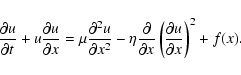 |
(60) |
An issue closely related to this problem is the behavior of the
correction to "dust'' concerning the local "energy budget''. The
density of mean peculiar-kinetic energy is defined as
![]() .
From Eqs. (13) one finds:
.
From Eqs. (13) one finds:
In the "SSE model'', the sign of the work done by the deviations from
mean field gravity,
![]() ,
depends on the orientation of the tidal tensor
and, like the work done by mean field gravity, is
in general unrelated to whether the fluid is locally compressing or
expanding. On the other hand, the work done by velocity dispersion is
most easily expressed in the basis that diagonalizes the symmetric
part of
,
depends on the orientation of the tidal tensor
and, like the work done by mean field gravity, is
in general unrelated to whether the fluid is locally compressing or
expanding. On the other hand, the work done by velocity dispersion is
most easily expressed in the basis that diagonalizes the symmetric
part of
![]() (this is
(this is
![]() ,
according to the decomposition (21)):
,
according to the decomposition (21)):
Starting from the equations of motion for point particles, we have implemented a smoothing procedure in phase space leading to equations for the smoothed density and peculiar-velocity fields in Eulerian space. These equations are the first ones in an infinite hierarchy of equations, and approximations to close the hierarchy are required. A closure approximation corresponds physically to an ansatz on how the evolution of the filtered fields is coupled to the degrees of freedom below the filtering scales. In this unified context, we have addressed three different closures, leading to three different models proposed earlier in the literature: the "dust model'', the "EJN model'', and the "SSE model''. The "dust model'' describes the evolution of fluid volume elements under the sole influence of the self-consistently generated gravitational field. The corrections to "dust'' take into account the dynamical influence of the small-scale degrees of freedom. The "EJN model'' approximates this influence as a density-dependent pressure. The "SSE model'' expresses this influence as a functional of density and velocity in a systematic expansion.
We have provided a clear explanation of how the corrections to the "dust model'' by both the "EJN closure'' and the "SSE closure'' lead to models that are qualitatively equivalent to the "adhesion model''. The key hypothesis is the parallelism relation (24) between peculiar-velocity and peculiar-acceleration. This already holds in Zel'dovich's approximation to the exact "dust'' evolution - the assumption underlying the "adhesion approximation'' consists of extrapolating it to also evaluate the corrections to "dust''.
We have shown that within both the Eulerian and Lagrangian perturbation frameworks, the corrections to "dust'' violate this assumption in general. Going beyond the phenomenology of the "adhesion model'' therefore requires relaxing of the parallelism assumption. When this is done, differences between the "EJN model'' and the "SSE model'' appear: deviations from the parallelism relationship arise at linear (both Eulerian and Lagrangian) perturbative order in the "EJN model'', but not in the "SSE model''; vorticity is generated by the "SSE''-corrections to "dust'', but not by the "EJN''-corrections.
The non-perturbative theoretical investigation raises considerable
difficulties. We suggested the plane-symmetric case as the "exact body'' of
the non-perturbative equations that may serve as a starting point for
a deeper understanding of the presented models.
This case can be reduced to the study of a single partial
differential equation for the displacement field, offering the possibility to
study the "EJN'' and "SSE'' models beyond any approximation.
This simplification misses some features that are expected to be of
relevance for the detailed inner structure of collapsing high-density
regions (e.g., generation of vorticity or the fact that velocity and
gravity have different directions).
We suggested a new non-perturbative approximation, which
yields a hybrid Eulerian/Lagrangian partial differential equation for the displacement field
that contains
as limits (i) the Eulerian and Lagrangian linear approximations,
and (ii) the standard "adhesion approximation'' if one
imposes the assumption of parallelism of peculiar-velocity and -acceleration.
When particularized to the "EJN model'', the "virial equation of state''
![]() provides substantial simplifications and, at the same time, is
a reasonable choice. We argued how this approximation can be viewed as the next step beyond the
parallelism assumption required by the "adhesion model''.
Finally, we provided a qualitative discussion of the exact "EJN''
and "SSE'' models concerning the formation of singularities.
provides substantial simplifications and, at the same time, is
a reasonable choice. We argued how this approximation can be viewed as the next step beyond the
parallelism assumption required by the "adhesion model''.
Finally, we provided a qualitative discussion of the exact "EJN''
and "SSE'' models concerning the formation of singularities.
An issue we have not addressed in this work is the choice of the smoothing scale L. This must be guided by the expected applicability of the corresponding closure approximations, in turn likely related to the initial conditions. The investigation of this point seems to require first the ability to extract predictions from the new models in order to validate them with respect to observations and viable N-body simulations.
Further exploration and numerical realization of the models
presented will hopefully lead us not only to approaches capable
of following large-scale structure into the non-linear regime, but
will also offer an interesting way of understanding the role of
previrialization (Peebles & Groth 1976; Davis & Peebles 1977;
Peebles 1990; ![]() okas et al. 1996), and the onset of virialization
in connection with galaxy and galaxy cluster formation. Furthermore
such models can be employed to improve generic inhomogeneous
collapse models (Buchert et al. 2000; Kerscher et al. 2001), and to
enhance the power of reconstructions of initial data from present-day
density and peculiar-velocity fields
(e.g., Croft & Gaztañaga 1997; Brenier et al.
2003; Mohayaee et al. 2003
for recent efforts). In the latter context, the proposed non-perturbative approximation,
based on the relation
okas et al. 1996), and the onset of virialization
in connection with galaxy and galaxy cluster formation. Furthermore
such models can be employed to improve generic inhomogeneous
collapse models (Buchert et al. 2000; Kerscher et al. 2001), and to
enhance the power of reconstructions of initial data from present-day
density and peculiar-velocity fields
(e.g., Croft & Gaztañaga 1997; Brenier et al.
2003; Mohayaee et al. 2003
for recent efforts). In the latter context, the proposed non-perturbative approximation,
based on the relation
![]() ,
Eq. (55), may provide an
alternative to the assumption of parallelism of peculiar-acceleration and
peculiar-velocity,
,
Eq. (55), may provide an
alternative to the assumption of parallelism of peculiar-acceleration and
peculiar-velocity,
![]() ,
Eq. (24).
,
Eq. (24).
Acknowledgements
This work was motivated by an exciting workshop at Observatoire de la Côte d'Azur (OCA) on the present subject with financial support by OCA, the French Ministry of Education, the Programme National de Cosmologie and the Laboratoire G. D. Cassini. Particular thanks to Uriel Frisch for organizing this workshop. Fruitful discussions were held with him, Erik Aurell, Stéphane Colombi, José Gaite, Sergei Gurbatov, Roman Juszkiewicz, Roya Mohayaee, Sergei Shandarin, Andrei Sobolevski, Alexei Starobinsky, Takayuki Tatekawa, Roland Triay, Patrick Valageas and Barbara Villone. T.B. acknowledges support by the "Sonderforschungsbereich SFB 375 für Astro-Teilchenphysik der Deutschen Forschungsgemeinschaft'', and by CERN, Geneva, where a preliminary manuscript was written during a visit of TB in 1998. A.D. acknowledges financial support by the project "Formación de estructuras en astrofísica y cosmología'' (BFM2002-01014) of the Spanish government.
To derive Eqs. (13) we first introduced comoving
coordinates, Eqs. (10), and then the coarse-graining procedure was applied.
It is legitimate to ask whether the order can be exchanged, i.e., what
are the transformations that lead from Eqs. (8) to
Eqs. (13)? They can be obtained easily by inserting the
transformations (10) into the
definitions (12), (14) and using the
definitions (7), (9).
One gets (here we write explicitly the dependence on the smoothing
length):
| (A.1b) |
| (A.1c) |
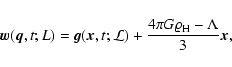 |
(A.1d) |
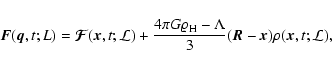 |
(A.1e) |
| (A.1f) |
The following new quantities had to be introduced:
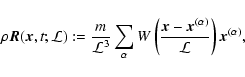 |
(A.2a) |
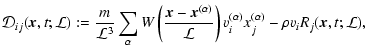 |
(A.2b) |
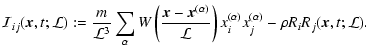 |
(A.2c) |
Compared to this "standard transformation'',
transformation (A.1) differs in two points: (i) the
additional transformation rules (A.1e,f) involving
the fields ![]() and
and
![]() ,
and (ii) the transformation between
,
and (ii) the transformation between ![]() and
and ![]() ,
because in general
,
because in general
![]() .
When the particle distribution looks
homogeneous at all cosmological scales, the deviation
.
When the particle distribution looks
homogeneous at all cosmological scales, the deviation
![]() is
irrelevant. In the highly non-linear regime of large inhomogeneities, one
expects
is
irrelevant. In the highly non-linear regime of large inhomogeneities, one
expects
![]() ,
but then
,
but then
![]() nevertheless, and
the cosmological expansion is also irrelevant (Domínguez & Gaite 2001). The
difference may be important in the most interesting case when the
structure is beginning to enter the non-linear regime,
nevertheless, and
the cosmological expansion is also irrelevant (Domínguez & Gaite 2001). The
difference may be important in the most interesting case when the
structure is beginning to enter the non-linear regime,
![]() .
.
Although the change to comoving coordinates does not affect the physical content of the resulting equivalent Eqs. (8) or (13), this equivalence can be broken after approximations are made. It seems more straightforward to "subtract'' the known background cosmological expansion before performing any smoothing/averaging, as we did to derive Eqs. (13), so that the approximations are concerned only with the "unknown'' part of the evolution of the inhomogeneities. However, the above remarks show that this procedure "hides'' additional physics and requires a careful definition of "background'' at the coarse-graining scale, which is only implicit by coarse-graining in the pre-defined comoving space.
In this Appendix we recall the derivation of the "SSE''
closure (19) (Domínguez 2000).
In analogy with definitions (12), one can formally
define microscopic fields by integrating the Klimontovich density (3)
over the velocity variable![]() :
:
| |
:= | ||
| = | (B.1a) |
| |
:= | ||
| = | (B.1b) |
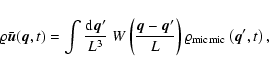 |
(B.3b) |
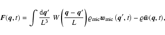 |
(B.3c) |
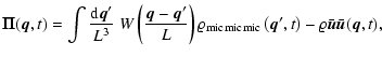 |
(B.3d) |
where
![]() is the mean-field strength of the peculiar-gravity,
defined by Eqs. (13c,d). The introduction of the
mic-fields is a formal step to express the definitions in terms
of volume integrals over fields.
Notice in particular that
is the mean-field strength of the peculiar-gravity,
defined by Eqs. (13c,d). The introduction of the
mic-fields is a formal step to express the definitions in terms
of volume integrals over fields.
Notice in particular that ![]() is defined by a volume-average of the
peculiar-momentum density (i.e., by a mass-average of the
velocity) and thus it has the physical meaning of center-of-mass
velocity of the coarsening cell. These fields obey
Eqs. (B.3a,b), which can be formally inverted to yield the following
expansion in L (this is most easily derived in Fourier space; this
formal inversion is defined provided the Fourier transform of the
window
is defined by a volume-average of the
peculiar-momentum density (i.e., by a mass-average of the
velocity) and thus it has the physical meaning of center-of-mass
velocity of the coarsening cell. These fields obey
Eqs. (B.3a,b), which can be formally inverted to yield the following
expansion in L (this is most easily derived in Fourier space; this
formal inversion is defined provided the Fourier transform of the
window ![]() has no zeros):
has no zeros):
![\begin{displaymath}%
\bu_{{\rm mic}} = \left[ 1 - \frac{1}{2} B ~ \left(L ~ \nab...
...ft(L ~
\nabla_{{\vec{q}}}\right)^4 \right] ~ \bar{\vec{u}},
\end{displaymath}](/articles/aa/full/2005/29/aa2885-05/img371.gif) |
(B.4b) |
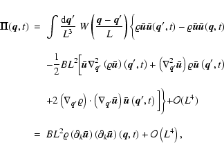
An ingredient of the "EJN'' model is an "equation of
state''![]()
![]() for the trace of the velocity dispersion tensor as
function of the mass density, Eq. (16). In this
appendix we summarize the evidence in favor of this assumption and the
physical meaning of some particular functional dependences.
for the trace of the velocity dispersion tensor as
function of the mass density, Eq. (16). In this
appendix we summarize the evidence in favor of this assumption and the
physical meaning of some particular functional dependences.
The density-dependence of the trace of the velocity
dispersion (14b) was addressed systematically with
N-body simulations of CDM scenarios by Domínguez (2003) and
Domínguez & Melott (2004) and can be summarized in a (sometimes
piecewise) polytropic dependence
![]() ,
which should be understood as an average, because
the numerical data scatter around this dependence.
The index
,
which should be understood as an average, because
the numerical data scatter around this dependence.
The index ![]() is always found to lie in the range
is always found to lie in the range
![]() .
The more power there is in the small scales of
the initial mass distribution relative to the large scales, the
smaller is
.
The more power there is in the small scales of
the initial mass distribution relative to the large scales, the
smaller is ![]() .
.
There are values of the index ![]() which have a
particular significance (see also Buchert et al. 1999):
which have a
particular significance (see also Buchert et al. 1999):
This model is frequently encountered in our paper. From a
mathematical point of view, the index ![]() entails a
simplification because the length
entails a
simplification because the length
![]() ,
Eq. (18), becomes
,
Eq. (18), becomes ![]() -independent. Thus, the
standard "adhesion model'' is recovered in this case because the GM coefficient
-independent. Thus, the
standard "adhesion model'' is recovered in this case because the GM coefficient ![]() ,
Eq. (26), is also
,
Eq. (26), is also ![]() -independent; see also the derivation of
Eq. (57).
-independent; see also the derivation of
Eq. (57).
Physically, one can argue on the basis of the virial theorem
(e.g. Chandrasekhar & Lee 1968): a well-known
consequence of it is that, if a system dominated by gravity is
isolated and in a stationary state, then the total
kinetic energy ![]() (in the frame of the system's center of
mass) and the total (gravitational) potential energy
(in the frame of the system's center of
mass) and the total (gravitational) potential energy ![]() are
related by the equation
are
related by the equation
![]() .
If our system is
a coarsening cell of size
.
If our system is
a coarsening cell of size ![]() L defined by the smoothing
window
L defined by the smoothing
window ![]() ,
we have
,
we have
![]() and
and
![]() assuming that
assuming that ![]() can be estimated reliably
within a mean field approximation (i.e., not too much small-scale
structure). To the extent that a coarsening cell can be considered
approximately isolated and stationary, the virial theorem implies
can be estimated reliably
within a mean field approximation (i.e., not too much small-scale
structure). To the extent that a coarsening cell can be considered
approximately isolated and stationary, the virial theorem implies
![]() .
The use of this relationship in the evolution
Eq. (17b) always supposes an approximation, because the
term
.
The use of this relationship in the evolution
Eq. (17b) always supposes an approximation, because the
term ![]() represents the flux of momentum by the exchange of
particles between neighboring coarsening cells, in contradiction with
the assumption of isolation required to derive the dependence
represents the flux of momentum by the exchange of
particles between neighboring coarsening cells, in contradiction with
the assumption of isolation required to derive the dependence
![]() .
.
In this case, the plane-symmetric problem of the "EJN model'', in the absence of cosmological expansion, can be mapped exactly to the "Sine-Gordon equation'' (Götz 1988).
Physically, this dependence implies that the kinetic energy per
particle, which is proportional to ![]() ,
is
density-independent. In the context of a fluid in thermal
equilibrium, the reason is that, concerning any single particle, the
rest of the system behaves like a thermostat.
,
is
density-independent. In the context of a fluid in thermal
equilibrium, the reason is that, concerning any single particle, the
rest of the system behaves like a thermostat.
Starting from the definition (14b), one can compute
the following evolution equation for the tensor ![]() :
:
The coefficient of proportionality ![]() is a local
function of the Lagrangian coordinates given by the initial data;
if we assume that, initially, this function is a spatial constant,
then we are entitled to talk about a "state'', since the relation
between dynamical "pressure'' and mass density is then global.
is a local
function of the Lagrangian coordinates given by the initial data;
if we assume that, initially, this function is a spatial constant,
then we are entitled to talk about a "state'', since the relation
between dynamical "pressure'' and mass density is then global.
In a plane-symmetric configuration, Eq. (C.1) can be
integrated under the assumption that
![]() and
and
![]() are negligible without the need for the additional isotropy
ansatz for
are negligible without the need for the additional isotropy
ansatz for ![]() .
Thus, the equation for the single component
.
Thus, the equation for the single component ![]() becomes
becomes
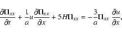
Without regard to this derivation, in the
context of the generalized "adhesion models'', the ![]() -dependence of the GM coefficient derived with the "SSE model'', Eq. (28), can be obtained
with the "EJN model'' and a dependence
-dependence of the GM coefficient derived with the "SSE model'', Eq. (28), can be obtained
with the "EJN model'' and a dependence
![]() ,
Eq. (26).
,
Eq. (26).
If one looks for a solution of Eqs. (17) in "comoving
hydrostatic equilibrium'', i.e.,
![]() but
but
![]() ,
with an "equation of state''
,
with an "equation of state''
![]() ,
then one can easily check that
,
then one can easily check that
![]() is the only possible
index for which a solution exists when
is the only possible
index for which a solution exists when ![]() is
time-independent (Chandrasekhar 1967).
is
time-independent (Chandrasekhar 1967).
In our context, this formal case is of interest because the
particularization of the "EJN model'' to a plane-symmetric
configuration gives a linear equation for the Lagrangian
displacement field ![]() exactly, see Sect. 6.2.
exactly, see Sect. 6.2.
More generally, the index ![]() introduces
mathematical simplifications in the integration of Euler's equation.
Recently, the Chaplygin gas has received attention in
cosmological research as one possible model of dark energy (see
e.g. the recent preprint by Gorini et al. 2004, and
refs. therein).
introduces
mathematical simplifications in the integration of Euler's equation.
Recently, the Chaplygin gas has received attention in
cosmological research as one possible model of dark energy (see
e.g. the recent preprint by Gorini et al. 2004, and
refs. therein).
Application of boundary-layer theory to Eqs. (26)
(Domínguez 2000) shows that density singularities are
regularized when ![]() .
On the other hand, a similar analysis
(Domínguez, unpublished) demonstrates that "pressure'' is too
weak to avoid the occurrence of singularities when
.
On the other hand, a similar analysis
(Domínguez, unpublished) demonstrates that "pressure'' is too
weak to avoid the occurrence of singularities when ![]() .
.
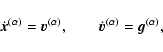
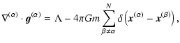
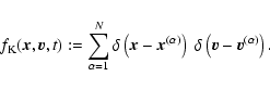
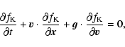
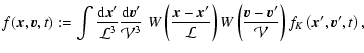
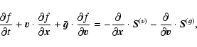
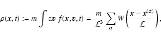
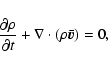
![$\displaystyle \frac{m}{{\cal L}^3} \sum_\alpha
W \left(\frac{{\vec{x}}-{\vec{x}...
...}}{{\cal L}} \right)
\left[ g_i^{(\alpha)} - {\bar g}_i ({\vec{x}}, t) \right],$](/articles/aa/full/2005/29/aa2885-05/img47.gif)
![$\displaystyle \nabla_{{\vec{q}}}^{(\alpha)} \cdot {\vec{w}}^{(\alpha)} = - 4 \p...
...\delta\left({\vec{q}}^{(\alpha)}-{\vec{q}}^{(\beta)}\right) -\varrho_H \right],$](/articles/aa/full/2005/29/aa2885-05/img76.gif)
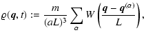
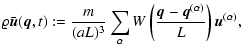
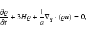
![\begin{displaymath}%
F_i ({\vec{q}}, t) := \frac{m}{(a L)^3} \sum_\alpha W
\le...
...\right)
\left[ w_i^{(\alpha)} - {w}_i ({\vec{q}}, t)\right],
\end{displaymath}](/articles/aa/full/2005/29/aa2885-05/img86.gif)
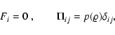
![\begin{displaymath}%
\lambda (\varrho) := \left[ \frac{p'(\varrho)}{4 \pi G \varrho}
\right]^{1/2}\cdot
\end{displaymath}](/articles/aa/full/2005/29/aa2885-05/img110.gif)
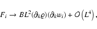
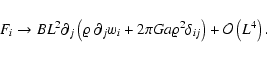
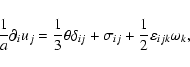
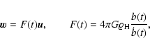
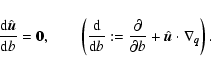
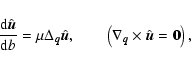
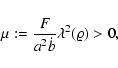
![\begin{displaymath}%
\frac{1}{\varrho} \left[ F_i - \frac{1}{a} \Pi_{ij,j} \righ...
...t(\partial_k u_i\right) \left(\partial_k u_j\right) \right].
\end{displaymath}](/articles/aa/full/2005/29/aa2885-05/img141.gif)
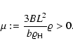
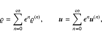
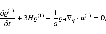

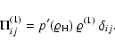
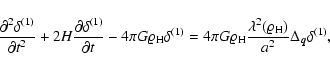
![$\displaystyle F (t) \left[ {\vec{u}}^{(1)} -
\frac{{\cal C}(t)}{a^2} \lambda^2\...
...right) \Delta_{\vec{q}}{\vec{u}}^{(1)}
+ {\cal O}\left(\lambda^4\right) \right]$](/articles/aa/full/2005/29/aa2885-05/img204.gif)
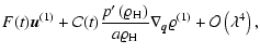
![$\displaystyle %
\frac{\partial \omega_i}{\partial t} + 2 H \omega_i + \frac{1}{...
...l_j \left[ \frac{1}{\varrho}
\left(F_k - \frac{1}{a} \Pi_{km,m}\right) \right].$](/articles/aa/full/2005/29/aa2885-05/img208.gif)
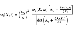
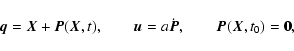
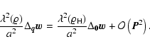
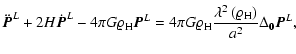
![$\displaystyle %
\ddot{{\vec{P}}} + 2 H \dot{{\vec{P}}} - 4 \pi G \varrho_{\rm H...
...varrho} \left[ {\vec{F}}- \frac{1}{a} \nabla_{\vec{q}}\cdot {\vec{\Pi}}\right].$](/articles/aa/full/2005/29/aa2885-05/img261.gif)
![$\displaystyle \ddot \Delta + 2 H \dot \Delta - 4\pi G \varrho_{\rm H} \Delta =
...
...vec{F}}-
\frac{1}{\varrho a}{\nabla}_{{\vec{q}}}\cdot{\vec{\Pi}}\right)\right],$](/articles/aa/full/2005/29/aa2885-05/img266.gif)
![$\displaystyle \left[\frac{a_{0}}{a}\right]^3 \varrho ({\vec{X}}, t_{0}) ~
\frac{\det J_{ij} ({\vec{X}},t_{0})}{\det J_{ij} ({\vec{X}},t)}$](/articles/aa/full/2005/29/aa2885-05/img273.gif)
![$\displaystyle \varrho(X, t) = \varrho_{\rm H}(t) ~ \left[ 1 + \frac{\partial P(X,t)}{\partial X}
\right]^{-1},$](/articles/aa/full/2005/29/aa2885-05/img278.gif)
![$\displaystyle \frac{\partial}{\partial q} = \left[ 1 + \frac{\partial P(X,t)}{\partial X} \right]^{-1}
\frac{\partial}{\partial X},$](/articles/aa/full/2005/29/aa2885-05/img279.gif)
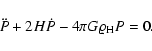
![\begin{displaymath}%
\ddot{{\vec{P}}} + 2 H \dot{{\vec{P}}} - 4 \pi G \varrho_{\...
...vec{F}}- \frac{1}{a} \nabla_{\vec{q}}\cdot {\vec{\Pi}}\right].
\end{displaymath}](/articles/aa/full/2005/29/aa2885-05/img294.gif)
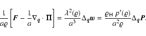
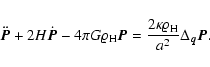
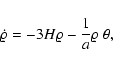
![\begin{displaymath}%
\varrho({\vec{X}}, t) = \varrho({\vec{X}}, t_{0}) ~ \left[...
...}\tau \; \frac{\theta ({\vec{X}}, \tau)}{a(\tau)} \right]\cdot
\end{displaymath}](/articles/aa/full/2005/29/aa2885-05/img305.gif)
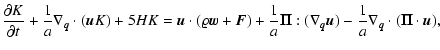
![$\displaystyle 2 B (a L)^2 \varrho \sum_i s_{(i)}
\left[ s_{(i)}^2
+ \frac{1}{4} \left(\omega^2-\omega_i^2\right) \right],$](/articles/aa/full/2005/29/aa2885-05/img323.gif)
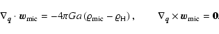
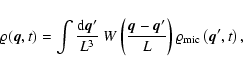
![\begin{displaymath}%
\varrho_{{\rm mic}} = \left[ 1 - \frac{1}{2} B ~ \left(L ~ ...
...al O}\left(L ~ \nabla_{{\vec{q}}}\right)^4 \right] ~ \varrho,
\end{displaymath}](/articles/aa/full/2005/29/aa2885-05/img370.gif)