J.-M. Grießmeier1 - U. Motschmann1 - G. Mann2 - H. O. Rucker3
1 - Institut für Theoretische Physik, Technische Universität
Braunschweig, Mendelssohnstraße 3, 38106 Braunschweig, Germany
2 -
Astrophysikalisches Institut Potsdam, An der Sternwarte 16, 14482 Potsdam, Germany
3 -
Institut für Weltraumforschung, Österreichische Akademie der Wissenschaften, Schmiedlstrasse 6, 8042 Graz, Austria
Received 8 September 2004 / Accepted 21 February 2005
Abstract
Magnetized giant exoplanets in close orbits around their host star
are expected to be strong nonthermal radio emitters.
The anticipated radio flux is strong enough to allow its detection on Earth using the next
generation of instruments. However, the measured quantity will not be the planetary radio flux
but the sum of planetary and stellar emission.
We compare the expected stellar and planetary radio signal for stellar systems of different ages.
Solar-like stellar wind parameters as well as conditions corresponding to
the young solar system (i.e. with increased stellar wind density and velocity) are considered.
For young stellar systems, conditions appear to be more favorable than for older stellar
systems.
It is shown that configurations exist where the separation of the planetary signal from the
stellar emission seems feasible.
Key words: planetary systems - magnetic fields - radiation mechanisms: non-thermal - Sun: radio radiation - radio continuum: stars
When considering "direct detection'' of extrasolar planets, one has always to keep in mind that
it is at present
not possible to resolve an extrasolar planetary system. Thus an observer will always see the
combined signal of the central star and of the planet(s). This is true for observations in all spectral
ranges, but the intensity ratio of stellar to planetary emission varies.
From the calculation of theoretical spectra for wide-separation (>0.2 AU)
extrasolar giant planets, Burrows et al. (2004) deduce a flux ratio of ![]() 108 in the
visible range and
108 in the
visible range and ![]() 104 for infrared emission. For closer separations, they find a
flux ratio of 103 for the mid-infrared.
The situation is different for the low-frequency radio range. Planetary radio emission is
dominated by powerful nonthermal emission
generated by the cyclotron-maser-instability (CMI). The solar radio emission
- which will serve as the main example of stellar radio emission throughout this paper -
consists of a quiet background (produced by thermal bremsstrahlung) plus a rich
spectrum of radio bursts (caused by nonthermal electrons).
The difference in generation mechanism allows for a much more favorable intensity ratio in the
spectral range considered here, thus making it easier to separate the stellar and the planetary
radio emission, as will be explained in detail below.
104 for infrared emission. For closer separations, they find a
flux ratio of 103 for the mid-infrared.
The situation is different for the low-frequency radio range. Planetary radio emission is
dominated by powerful nonthermal emission
generated by the cyclotron-maser-instability (CMI). The solar radio emission
- which will serve as the main example of stellar radio emission throughout this paper -
consists of a quiet background (produced by thermal bremsstrahlung) plus a rich
spectrum of radio bursts (caused by nonthermal electrons).
The difference in generation mechanism allows for a much more favorable intensity ratio in the
spectral range considered here, thus making it easier to separate the stellar and the planetary
radio emission, as will be explained in detail below.
For most of the discussion we will assume the star to be similar to the sun. In Sect. 2.2 a type of stellar radio emission which does not exist on the sun is presented. For close-in extrasolar giant planets much higher flux densities are expected when compared to the radio planets of the solar system (e.g. Farrell et al. 1999; Zarka et al. 2001). These estimations are reviewed and revised in this work; in addition, we show that the temporal evolution of the stellar wind as presented by Grießmeier et al. (2004) has to be taken into account. We also compare our results to those of the recent study of Lazio et al. (2004).
In Sect. 2 we will treat different kinds of solar (Sect. 2.1) and stellar (Sect. 2.2) radio emission. Section 3 briefly describes the flux density spectrum of Jupiter (Sect. 3.1) and discusses the radio flux expected from different extrasolar planets under present-day stellar wind conditions (Sect. 3.2). Section 4 expands this discussion by taking into account the stellar wind evolution with time. It will be shown how this affects planetary radio emission. In Sect. 5 the stellar and planetary flux densities are compared. Section 6 closes with a few concluding remarks.
The solar radio flux is composed of different components, not all of which are always present. The components differ in intensity and rate of occurrence and are caused by different emission mechanisms. Three different emission mechanisms are important (Warmuth & Mann 2005):
![\begin{figure}
{\includegraphics[width=8.8cm,clip]{1976fig1.ps} }
%
\end{figure}](/articles/aa/full/2005/26/aa1976-04/img4.gif) |
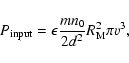
Figure 1: Solar radio spectrum according to Boischot & Denisse (1964) (dotted line) and Nelson et al. (1985) (solid lines). The quiescent stellar emission of the dG0e star HD 129333 (=EK Dra) measured at 8.4 GHz (Güdel et al. 1995) as well as that of the dM5.5e star UV Cet (short dashed line, from Güdel & Benz 1996) are normalized to a distance of 1 AU for comparison (see Sect. 2.2). |
| Open with DEXTER | |
The quiet sun emission is caused by thermal bremsstrahlung due to electron-ion collisions in the ionized plasma. Observations at different frequencies typically yield information about different layers in the star. The higher the frequency f, the denser (and lower) the generating layer may have been. Most of the observed quiet sun radio emission comes from the solar atmosphere (and not from deep inside the sun).
The slowly varying component
(not shown in Fig. 1) is
mainly due to gyrosynchrotron emission from regions of hot and dense
plasma in the corona e.g. over sunspots (Warmuth & Mann 2005). This
leads to a flux density variation by a factor of ![]() 2 at centimetre and decimetre
wavelengths
(Sheridan & McLean 1985). It has a periodicity of 27 days due to
solar rotation (Boischot & Denisse 1964) and varies over the sunspot cycle. While the quiet sun emission
is randomly polarized (Sheridan & McLean 1985), the emission in the centimetric range is often
circularly polarized, which can only be explained by the strong magnetic fields of the sunspots
(Boischot & Denisse 1964).
2 at centimetre and decimetre
wavelengths
(Sheridan & McLean 1985). It has a periodicity of 27 days due to
solar rotation (Boischot & Denisse 1964) and varies over the sunspot cycle. While the quiet sun emission
is randomly polarized (Sheridan & McLean 1985), the emission in the centimetric range is often
circularly polarized, which can only be explained by the strong magnetic fields of the sunspots
(Boischot & Denisse 1964).
Solar radio bursts are generated by high-frequency plasma oscillations excited by suprathermal electrons. These plasma oscillations have to be converted into electromagnetic radiation. Solar radio bursts typically have much higher flux densities than the quiet sun emission. They are observed in the whole frequency range, but they are more intense in the low frequency domain (see Fig. 1). The emission takes place close to the electron plasma frequency or its harmonics (Melrose 1985).
Solar radio bursts are usually partially circularly polarized.
Some types of solar radio bursts are briefly presented in the following;
a more complete review is given by Warmuth & Mann (2005).
Type I bursts only occur in large groups. These Noise Storms are described below.
Type II bursts are generated by magnetohydrodynamic shock waves caused by a
disturbance moving with super-Alfvénic velocity. Suprathermal electrons in the shock-front
region excite Langmuir waves which are converted to electromagnetic radiation. Type II bursts
display a detailed fine structure (see e.g. Mel'nik et al. 2004).
Polarization is similar to type III bursts (see below).
Type III bursts, characteristic of
the impulsive phase of solar flares, are the most common flare-associated bursts.
They are generated by relativistic electrons (typically
![]() ,
see Warmuth & Mann 2005).
Because of the high particle velocity, a large frequency drift
,
see Warmuth & Mann 2005).
Because of the high particle velocity, a large frequency drift
![]() is a
characteristic feature of type III-Bursts. For this type of emission,
radio waves are emitted not only at the
fundamental frequency of plasma waves, but also at their second harmonic (Bougeret et al. 1984).
The polarization degree ranges from weak (<0.15) to moderately high (
is a
characteristic feature of type III-Bursts. For this type of emission,
radio waves are emitted not only at the
fundamental frequency of plasma waves, but also at their second harmonic (Bougeret et al. 1984).
The polarization degree ranges from weak (<0.15) to moderately high (![]() 0.5).
Non-flare related type III bursts are found in type III storms (see below).
The broadband emission of a
type IV burst is caused by energetic electrons trapped in a closed magnetic structure. Some of
these structures are stationary, others move slowly upward, leading to a slow frequency drift.
Type V bursts are continuum emissions over a wide frequency range. They follow
type III bursts and typically have the opposite circular polarization than the
preceding type III burst.
0.5).
Non-flare related type III bursts are found in type III storms (see below).
The broadband emission of a
type IV burst is caused by energetic electrons trapped in a closed magnetic structure. Some of
these structures are stationary, others move slowly upward, leading to a slow frequency drift.
Type V bursts are continuum emissions over a wide frequency range. They follow
type III bursts and typically have the opposite circular polarization than the
preceding type III burst.
Noise storms are frequently the dominant component of solar radio emission for wavelengths between 1 and 10 m. Both flare and non-flare related noise storms exist. Two types of storms are distinguished, which are named type I storms and type III storms after the type of radio bursts associated with them. Although the radio flux density associated with a type I noise storm is far below that of a radio burst, it can be 1000 times that of the quiet sun. Due to their occurrence rate and their duration, noise storms significantly contribute to the signal detected: near solar maximum, noise storms occur about 10% of the time (Hjellming 1988). The typical duration of a noise storm is between a few hours and several days (Boischot & Denisse 1964; Warmuth & Mann 2005). Type I noise storms consist of a slowly varying broadband continuum plus short-lived bursts. The emission of type I storms is highly circularly polarized (Boischot & Denisse 1964; Kai et al. 1985). Type III storms are not associated with flares; they are connected to type III bursts (see above). Type III storms can also include continuum emission in addition to bursts, but these continua only have a low intensity (Kai et al. 1985). There often is a temporal relationship between type I storms and type III storms, possibly due to a common exciting agent (Kai et al. 1985). Type III storms always have the same polarization as type I storms, but the degree of polarization is usually much lower for type III storms.
Some stars are continuously emitting much more energy at radio frequencies than the sun. These radio luminosities can be 2-3 orders of magnitudes higher than the quiet sun (Benz 1993). This kind of emission is probably due to nonthermal processes (possibly gyrosynchrotron emission of energetic electrons); to emphasize the different generation mechanism of this emission with respect to the quiet sun emission, the term quiescent radio emission was introduced. There is no corresponding radiation on the sun. The typical variation of the quiescent emission is about 50% on a time scale of hours, and it has a low degree of polarization (Benz 1993). Unfortunately, measurements of stellar radio spectra are limited to a few frequencies. Also, no data are available for frequencies below 1 GHz. Figure 1 shows a spectrum for the quiescent stellar emission of the dM5.5e star UV Ceti (Güdel & Benz 1996, dataset 4), normalized to a distance of 1 AU. The stellar distance was taken to be 2.627 pc (calculated from Gliese & Jahreiß 1991). Güdel & Zucker (2000) fitted four-point VLA radio spectra to the gyrosynchrotron model of White et al. (1989). This fit indicates that for UV Cet, the maximum of the emission probably lies above 1 GHz, so that lower flux densities can be expected for lower frequencies. For frequencies below this maximum, theory predicts that the intensity is proportional to f2.5, while in reality exponents between 0 and 10 can be found (Benz 1993).
Also, stars with even higher quiescent radio flux exist. The quiescent radio flux decreases with increasing stellar age (Güdel et al. 1998). For this reason, the emission of a young star can serve as an upper limit for quiescent emission. Figure 1 shows the quiescent stellar emission of the young (approx. 70 Myr, see Dorren & Guinan 1994) dG0e star HD 129333 (=EK Draconis) as measured at the frequency of 8.4 GHz (Güdel et al. 1995), scaled to a distance of 1 AU. We will use the emission of HD 129333 as the upper limit to the contribution of the quiescent emission.
It is known that stellar flares can be much more energetic than solar flares; stellar flares with 104 times the radio flux of the largest solar radio burst have been observed. These flares are often completely circularly polarized (Benz 1993; Güdel et al. 1989). The influence of both stellar flares and quiescent radio emission on the detectability of planets is discussed in Sect. 5.
Some very large flares (up to 107 times more energetic than the largest solar flare) on solar-like stars could possibly be caused by the interaction of a normal G dwarf and a magnetized close-in extrasolar planet (Rubenstein & Schaefer 2000). However, so far only nine of these transient extreme events have been detected (Schaefer et al. 2000). For this reason, they do not present a systematic problem for the discrimination of stellar and planetary radio emission.
The first measurement of Jupiter's radio emission (the strongest planetary radio emission we
know) was made by Burke & Franklin (1955) at a frequency of 22 MHz.
Due to the Earth's ionosphere, frequencies below ![]() 5-10 MHz (Zarka et al. 1997) are not
accessible to ground-based observations. This explains why radio emissions from other planets
of the solar system (including the radio emission from the Earth's magnetosphere)
were unknown at that time. The full radio spectrum of Jupiter
could only be determined years later by the PRA experiment on both Voyager spacecraft
(Zarka 1992). About two days of Voyager data (obtained from a distance of 100-500 planetary radii)
were used to compute the spectrum, which was first published in 1992. Recently, the spectrum was
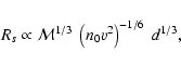
recalculated with much more accuracy using Cassini-RPWS data (Zarka et al. 2004).
Figure 2 is based on that spectrum. Unfortunately, Cassini-RWPS data are only
available for
5-10 MHz (Zarka et al. 1997) are not
accessible to ground-based observations. This explains why radio emissions from other planets
of the solar system (including the radio emission from the Earth's magnetosphere)
were unknown at that time. The full radio spectrum of Jupiter
could only be determined years later by the PRA experiment on both Voyager spacecraft
(Zarka 1992). About two days of Voyager data (obtained from a distance of 100-500 planetary radii)
were used to compute the spectrum, which was first published in 1992. Recently, the spectrum was
recalculated with much more accuracy using Cassini-RPWS data (Zarka et al. 2004).
Figure 2 is based on that spectrum. Unfortunately, Cassini-RWPS data are only
available for ![]() MHz. For higher frequencies, spectral data from Zarka et al. (1995) are
shown, corresponding to periods of intense activity (Zarka et al. 2004).
It can be seen that the peak flux
densities can be up to 100 times the average values. The observed spectrum is highly
time-dependent, e.g. through solar wind variability (Gurnett et al. 2002) and also
depends on the observer's position (due to beaming effects). To facilitate the comparison
with the solar radio emission of Sect. 2, the flux density scale
is normalized to 1 AU distance.
MHz. For higher frequencies, spectral data from Zarka et al. (1995) are
shown, corresponding to periods of intense activity (Zarka et al. 2004).
It can be seen that the peak flux
densities can be up to 100 times the average values. The observed spectrum is highly
time-dependent, e.g. through solar wind variability (Gurnett et al. 2002) and also
depends on the observer's position (due to beaming effects). To facilitate the comparison
with the solar radio emission of Sect. 2, the flux density scale
is normalized to 1 AU distance.
![\begin{figure}
{\includegraphics[width=8.8cm,clip]{1976fig2.ps} }\end{figure}](/articles/aa/full/2005/26/aa1976-04/img9.gif) |
Figure 2: Jupiter radio spectrum based on Cassini RPWS data (Zarka et al. 2004), normalized to a distance of 1 AU. Solid line: rotation averaged emission. Dashed line: rotation averaged emission at times of intense activity. Dotted line: peak intensities during active periods. The high-frequency data are taken from Zarka et al. (1995) and correspond to times of intense emission (see Zarka et al. 2004). |
| Open with DEXTER | |
The high frequency cutoff in the spectrum shown in Fig. 2 can be explained as follows. Typically, the source region is located between 2 and 4 planetary radii. It has been found that the radio emission is produced close to the local electron gyrofrequency along auroral fieldlines. Thus, the highest frequency emission will be generated at the location with the strongest magnetic field, i.e. closest to the planet's surface. This yields the "high-frequency cutoff'' around 40 MHz in Fig. 2. A more complete discussion of the different components of Jupiter's radiation can be found in Zarka (1998), updated in Zarka et al. (2004). Note that planetary radio emission is strongly circularly polarized (Zarka 1998,1992).
Already before the discovery of the first extrasolar planet around a star in 1995 (Mayor & Queloz 1995), attempts were made to discover the radio emission of extrasolar planets. So far, however, these efforts have been unsuccessful (Winglee et al. 1986; Zarka et al. 1997; Bastian et al. 2000; Yantis et al. 1977; Lazio et al. 2004; Farrell et al. 2003). One of the many possible reasons for the current non-detection given by Bastian et al. (2000) is the lack of sensitivity in the appropriate frequency range. This will be verified in this subsection and in Sect. 4.
It is clear that the radio emission of a planet in an extrasolar planetary system can differ
considerably from Jupiter's radio emission. A planet in a close-in orbit (![]() AU) around
its central star (a so-called "Hot Jupiter'')
is subject to strong tidal dissipation, leading to gravitational locking on a very short
timescale (Seager & Hui 2002).
For a hypothetical Jupiter-like planet orbiting a solar twin at 0.05 AU, the synchronisation
timescale is approximately
AU) around
its central star (a so-called "Hot Jupiter'')
is subject to strong tidal dissipation, leading to gravitational locking on a very short
timescale (Seager & Hui 2002).
For a hypothetical Jupiter-like planet orbiting a solar twin at 0.05 AU, the synchronisation
timescale is approximately
![]() years.
For gravitationally locked planets the rotation period is equal to the orbital period, and
fast rotation is not possible. Commonly employed scaling-laws for the planetary magnetic
moment (e.g. Grießmeier et al. 2004; Cain et al. 1995)
always yield a magnetic moment rapidly decreasing with decreasing
rotation rate. This influence of tidal locking on the planetary magnetic moment is examined
in detail by Grießmeier et al. (2004).
years.
For gravitationally locked planets the rotation period is equal to the orbital period, and
fast rotation is not possible. Commonly employed scaling-laws for the planetary magnetic
moment (e.g. Grießmeier et al. 2004; Cain et al. 1995)
always yield a magnetic moment rapidly decreasing with decreasing
rotation rate. This influence of tidal locking on the planetary magnetic moment is examined
in detail by Grießmeier et al. (2004).
In Table 1 the planetary parameters required for the magnetic moment
estimation as well as the resulting magnetic moments (upper and lower limits) are compared for
those planets where the radius is either known (from transit observations)
or reasonably well constrained by theoretical models (![]() Boo, see Burrows et al. 2000). This choice was made because
information on the planetary radius allows an improved estimation of the planetrary magnetic moment
(Grießmeier et al. 2004). The
quantities are given in units normalized to Jupiter
(denoted by subscript J), with
Boo, see Burrows et al. 2000). This choice was made because
information on the planetary radius allows an improved estimation of the planetrary magnetic moment
(Grießmeier et al. 2004). The
quantities are given in units normalized to Jupiter
(denoted by subscript J), with
![]() km,
km,
![]() kg,
kg,
![]() s-1,
s-1,
![]() Am2.
The planetary radius R and mass M was taken from
Cody & Sasselov (2002) for HD 209458b, from Torres et al. (2004) for OGLE-TR-56b,
from Bouchy et al. (2004) for OGLE-TR-113b
and from Moutou et al. (2004) for OGLE-TR-132b.
For the mass of
Am2.
The planetary radius R and mass M was taken from
Cody & Sasselov (2002) for HD 209458b, from Torres et al. (2004) for OGLE-TR-56b,
from Bouchy et al. (2004) for OGLE-TR-113b
and from Moutou et al. (2004) for OGLE-TR-132b.
For the mass of ![]() Boo only the lower limit is known
(
Boo only the lower limit is known
(
![]() ,
Leigh et al. 2003),
and the radius is presently not accessible to measurement.
Theoretical models by Burrows et al. (2000) yield an upper limit for the
radius of
,
Leigh et al. 2003),
and the radius is presently not accessible to measurement.
Theoretical models by Burrows et al. (2000) yield an upper limit for the
radius of
![]() for a planetary mass of
for a planetary mass of
![]() and of
and of
![]() for
a mass of
for
a mass of
![]() .
The most probable radius
seems to be
.
The most probable radius
seems to be
![]() (Leigh et al. 2003).
Because of this uncertainty, we
calculate the magnetic moment for three different cases:
a relatively "light'' planet (
(Leigh et al. 2003).
Because of this uncertainty, we
calculate the magnetic moment for three different cases:
a relatively "light'' planet (
![]() and
and
![]() ),
a "medium'' planet (
),
a "medium'' planet (
![]() and
and
![]() ),
and a "heavy'' planet (
),
and a "heavy'' planet (
![]() and
and
![]() ).
For each of these three model cases, the upper and lower limit for the
magnetic moment
).
For each of these three model cases, the upper and lower limit for the
magnetic moment
![]() was calculated.
The highest upper limit (i.e. for the "heavy'' case) and the lowest lower
limit (i.e. for the "light'' case) are given in Table 1.
The value of
was calculated.
The highest upper limit (i.e. for the "heavy'' case) and the lowest lower
limit (i.e. for the "light'' case) are given in Table 1.
The value of ![]() was calculated from the orbital period assuming tidal locking.
The core density
was calculated from the orbital period assuming tidal locking.
The core density
![]() is proportional to the mean density
is proportional to the mean density
![]() of the planet
(
of the planet
(
![]() ).
See Grießmeier et al. (2004) for additional details.
).
See Grießmeier et al. (2004) for additional details.
The magnetic dipole moment values were obtained exactly as in Grießmeier et al. (2004).
For the magnetic moment scaling, the size of the dynamo-region ![]() is required. Two different
scaling laws were suggested for this quantity: one based only on the mass of the planet
(Curtis & Ness 1986) and one based on both planetary mass and radius (Grießmeier et al. 2004).
Both approaches lead to unphysical results for the case of
is required. Two different
scaling laws were suggested for this quantity: one based only on the mass of the planet
(Curtis & Ness 1986) and one based on both planetary mass and radius (Grießmeier et al. 2004).
Both approaches lead to unphysical results for the case of ![]() Bootes: one finds
Bootes: one finds
![]() .
In these cases, we
set
.
In these cases, we
set
![]() for all subsequent calculations.
This approach may seem arbitrary, but it is reasonable to assume a monotonous
increase in
for all subsequent calculations.
This approach may seem arbitrary, but it is reasonable to assume a monotonous
increase in
![]() with planetary mass M. Thus, the real value for
with planetary mass M. Thus, the real value for ![]() Boo will lie in the range
Boo will lie in the range
![]() ,
and the error made by assuming
,
and the error made by assuming
![]() is tolerable.
is tolerable.
Not only is the size of the magnetic moment and thus of the magnetosphere very different for a "Hot Jupiter''. Also, the stellar wind is much denser because of the close proximity of the star. Both these effects will have an influence on the radio power emitted from an extrasolar planet, as will be seen in the following.
Table 1: Parameters for some "Hot Jupiters''. The values used for the calculation of the magnetic moments are given in units normalized to Jupiter. The lower part shows the scaling results for a stellar system of 4.6 Gyr age: planetary dipole moment, total emitted radio power, radio flux at 1 AU from the planet, radio flux at Earth (distance s) and maximum frequency. Values calculated for Jupiter are given for comparison. Sources of parameters: (a) Burrows et al. (2003), (b) Konacki et al. (2003), (c) Melo et al. (2004), (d) Moutou et al. (2004), (e) Leigh et al. (2003), (f) Cody & Sasselov (2002), (g) Torres et al. (2004), (h) Bouchy et al. (2004). See text for details.
A simple way to estimate the total emitted radio power of
planets within the solar system was originally suggested by Desch & Kaiser (1984).
This idea was later applied to the expected radio emission from extrasolar planets by Farrell et al. (1999).
The total power emitted in the radio range,
![]() ,
is probably roughly proportional to the total power incident
on the magnetosphere,
,
is probably roughly proportional to the total power incident
on the magnetosphere,
![]() (Zarka et al. 2001):
(Zarka et al. 2001):
The energy input into the magnetosphere is proportional to the cross-section of the
magnetosphere as seen from the star, determined by the magnetospheric radius ![]() :
:
The magnetospheric radius is determined from the pressure balance at the substellar point, i.e.
According to observations and models,
![]() for Jupiter (Joy et al. 2002). As a first-order approximation, self-similarity is satisfied (Vogt & Glassmeier 2001), so that a fixed ratio can be assumed for all planets:
for Jupiter (Joy et al. 2002). As a first-order approximation, self-similarity is satisfied (Vogt & Glassmeier 2001), so that a fixed ratio can be assumed for all planets:
![]() .
Note that in one case (for HD 209458b with
.
Note that in one case (for HD 209458b with
![]() ),
we obtained
),
we obtained
![]() .
In that case we set
.
In that case we set
![]() for all further calculations, because the magnetosphere cannot be compressed to sizes smaller than the planetary radius.
for all further calculations, because the magnetosphere cannot be compressed to sizes smaller than the planetary radius.
The fact that
![]() together with Eqs. (5) and (2)
can then be inserted into
Eq. (1), resulting in
together with Eqs. (5) and (2)
can then be inserted into
Eq. (1), resulting in
The total emitted power is now normalized to the radio power emitted by the planet Jupiter, so that
Eq. (6) becomes
From the total emitted radio power, the radio flux at a given distance can be calculated. Similarly to
Farrell et al. (1999) we calculate the radio flux as
 |
(9) |
If we compare our results for ![]() Bootes with the result of Farrell et al. (1999, Table 1),
we can see that in the present work the total radio power is smaller by a factor of
Bootes with the result of Farrell et al. (1999, Table 1),
we can see that in the present work the total radio power is smaller by a factor of ![]() 4,
while the flux is higher by a factor of
4,
while the flux is higher by a factor of ![]() 4. The values for the radio power
differ because of the different magnetic moments, while the flux densities are different
because we use a different magnetic moment, a smaller value of
4. The values for the radio power
differ because of the different magnetic moments, while the flux densities are different
because we use a different magnetic moment, a smaller value of
![]() and a smaller value for
and a smaller value for ![]() .
Thus, for average conditions, the results are approximately comparable.
While in Farrell et al. (1999) variations of
.
Thus, for average conditions, the results are approximately comparable.
While in Farrell et al. (1999) variations of ![]() and of stellar wind velocity are suggested to
potentially increase the total radio flux by up to three orders of magnitude, we believe that the
peak power will not be more than one order of magnitude above the value given in
Table 1 (e.g. if
and of stellar wind velocity are suggested to
potentially increase the total radio flux by up to three orders of magnitude, we believe that the
peak power will not be more than one order of magnitude above the value given in
Table 1 (e.g. if
![]() W is used
rather than
W is used
rather than
![]() W).
For this reason, the peak radio power (and the peak radio flux) differ considerably.
Note that so far, stellar wind conditions corresponding to a stellar system age of
4.6 Gyr were compared. The correct age
will be taken into account in Sect. 4.
W).
For this reason, the peak radio power (and the peak radio flux) differ considerably.
Note that so far, stellar wind conditions corresponding to a stellar system age of
4.6 Gyr were compared. The correct age
will be taken into account in Sect. 4.
In comparison to the recent study of Lazio et al. (2004) we note that Table I of that work
gives the peak power, while we use the average power during periods of high intensity.
Lazio et al. (2004) take the peak power to be two order of magnitude above average, leading
to a peak emission power much larger than that of the current study.
As far as the maximum emission frequency is concerned, we note that the frequency given
by Lazio et al. (2004) is higher by a factor of 3. This is due to the fact that they
use the magnetic moment scaling of Blackett (1947), which was
later experimentally disproved (Blackett 1952).
Due to the larger exponent in r, Blackett's laws leads to an overestimation of the
planetary magnetic moment for large planets. In addition, Lazio et al. (2004)
make use of the mass-radius relation
![]() .
Especially for planets with large masses like
.
Especially for planets with large masses like ![]() Boo,
this produces unrealistically large
planetary radii, magnetic moments, radio fluxes and emission frequencies.
Note that a good estimation of the emission frequency is particularly important
because a difference of a small factor can make the difference between radiosignals above and
below the ionospheric cutoff.
Boo,
this produces unrealistically large
planetary radii, magnetic moments, radio fluxes and emission frequencies.
Note that a good estimation of the emission frequency is particularly important
because a difference of a small factor can make the difference between radiosignals above and
below the ionospheric cutoff.
The radio flux ![]() from Table 1 has to be compared to the detection
limit of various radio-telescopes:
the UTR-2 detector in Kharkov presently has a sensitivity of 25 Jy (e.g. Rucker 2002).
This detector will be improved in the near future using modern digital techniques,
where a new backend facility
called Robin 2 (Rucker 2002) will improve the sensitivity down to 100 mJy. The
extremely ambitious project of a LOw Frequency ARray (LOFAR) will provide a sensitivity of 1 mJy
(Kassim et al. 2004).
from Table 1 has to be compared to the detection
limit of various radio-telescopes:
the UTR-2 detector in Kharkov presently has a sensitivity of 25 Jy (e.g. Rucker 2002).
This detector will be improved in the near future using modern digital techniques,
where a new backend facility
called Robin 2 (Rucker 2002) will improve the sensitivity down to 100 mJy. The
extremely ambitious project of a LOw Frequency ARray (LOFAR) will provide a sensitivity of 1 mJy
(Kassim et al. 2004).
It can be seen that the radio flux from the planet HD 209458b could in
principle be detectable
by LOFAR, but that the frequency is below the ionospheric cutoff. The reason for this is the weak
magnetic field due to synchronous rotation (tidal locking). The planets OGLE-TR-56b,
OGLE-TR-113b and OGLE-TR-132b are very far away. Even if the planets are relatively powerful
radio emitters and ionospheric cutoff is not a problem, the radio flux at Earth is much too low
to allow detection. Although these planets are not good candidates for radio observations, they
can serve as representatives of a certain class of planets. Note that non-transiting but otherwise similar
planets could exist much closer to the solar system. For such a planet, radio detection would be
possible. Finally,
it can be seen that the radio emission expected for
![]() Boo lies both above the ionospheric cutoff frequency and above the detection limit for
LOFAR, so that radio emission from that planet may be detectable in the near future.
Boo lies both above the ionospheric cutoff frequency and above the detection limit for
LOFAR, so that radio emission from that planet may be detectable in the near future.
Table 2:
Scaling output for a planet like ![]() Bootes at different stellar system
ages (4.6 Gyr, 1.0 Gyr and 0.7 Gyr). See text for details.
Bootes at different stellar system
ages (4.6 Gyr, 1.0 Gyr and 0.7 Gyr). See text for details.
Recently, stellar mass loss rates of main sequence G and K stars were
estimated by using recent indirect stellar wind observations (Wood et al. 2002).
This allowed the calculation of the stellar wind evolution (Grießmeier et al. 2004, Sect. 3.2);
this calculation was later limited to stellar systems with an
![]() Gyr (Lammer et al. 2004).
It could be shown that the stellar wind velocity of a young star (1 Gyr after reaching the main
sequence) is about twice as high as the velocity of today's solar wind (at 4.6 Gyr).
Likewise, the density of the stellar wind of a young G or K star is about one order of magnitude
higher. This has two effects: first, it compresses the magnetosphere, as can be seen from
Eq. (5). Secondly, the increased stellar wind parameters also increase the
energy input into the magnetosphere, see Eq. (2). It can be seen from
Eq. (7) that a denser and faster
stellar wind will lead to
stronger planetary radio emission.
This effect is important because the age of extrasolar planet host stars vary. For the star HD 209458,
an age of between 4 and 7 Gyr is assumed, with 5.2 Gyr as a likely value (Cody & Sasselov 2002; Mazeh et al. 2000).
For OGLE-TR-56 the age is given as
Gyr (Lammer et al. 2004).
It could be shown that the stellar wind velocity of a young star (1 Gyr after reaching the main
sequence) is about twice as high as the velocity of today's solar wind (at 4.6 Gyr).
Likewise, the density of the stellar wind of a young G or K star is about one order of magnitude
higher. This has two effects: first, it compresses the magnetosphere, as can be seen from
Eq. (5). Secondly, the increased stellar wind parameters also increase the
energy input into the magnetosphere, see Eq. (2). It can be seen from
Eq. (7) that a denser and faster
stellar wind will lead to
stronger planetary radio emission.
This effect is important because the age of extrasolar planet host stars vary. For the star HD 209458,
an age of between 4 and 7 Gyr is assumed, with 5.2 Gyr as a likely value (Cody & Sasselov 2002; Mazeh et al. 2000).
For OGLE-TR-56 the age is given as ![]() Gyr (Sasselov 2003).
Gyr (Sasselov 2003).
![]() Bootes has an age of approximately
Bootes has an age of approximately ![]() Gyr (Fuhrmann et al. 1998).
Using Eqs. (16) and (17) from Grießmeier et al. (2004) for v(t) and n(t), respectively,
and Eqs. (7) and (11) from above,
the total emitted radio power and the radio flux density are calculated and compared
in Table 2 for stellar system ages of 4.6 Gyr, 1.0 Gyr and 0.7 Gyr.
To facilitate the comparison, we also give v and n for the different cases.
The planetary radius, magnetic moment and semimajor axis are assumed to be constant, so that the
time evolution is caused by the variation of v and n.
Gyr (Fuhrmann et al. 1998).
Using Eqs. (16) and (17) from Grießmeier et al. (2004) for v(t) and n(t), respectively,
and Eqs. (7) and (11) from above,
the total emitted radio power and the radio flux density are calculated and compared
in Table 2 for stellar system ages of 4.6 Gyr, 1.0 Gyr and 0.7 Gyr.
To facilitate the comparison, we also give v and n for the different cases.
The planetary radius, magnetic moment and semimajor axis are assumed to be constant, so that the
time evolution is caused by the variation of v and n.
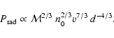
The lower limit for the radio flux expected from a planet like
![]() Bootes b at different stellar system ages as well as
the radio flux of Jupiter are compared in Fig. 3.
Note that if an age of 4.6 Gyr is assumed for
Bootes b at different stellar system ages as well as
the radio flux of Jupiter are compared in Fig. 3.
Note that if an age of 4.6 Gyr is assumed for ![]() Bootes, the expected radio flux
is underestimated by over one order of magnitude.
Concerning the current non-detection of radio emission from
Bootes, the expected radio flux
is underestimated by over one order of magnitude.
Concerning the current non-detection of radio emission from ![]() Bootes,
we suggest that the main problem is the
relatively low maximum frequency of 19 MHz of the emission as compared to the measurements at
Bootes,
we suggest that the main problem is the
relatively low maximum frequency of 19 MHz of the emission as compared to the measurements at
![]() MHz (Winglee et al. 1986; Bastian et al. 2000; Lazio et al. 2004; Farrell et al. 2003).
The observations of Zarka et al. (1997) are in a
more promising frequency range (between 7 and 35 MHz), but the sensitivity of the UTR-2
detector was not sufficient.
Similarly, the measurements by Yantis et al. (1977) were not sensitive enough.
MHz (Winglee et al. 1986; Bastian et al. 2000; Lazio et al. 2004; Farrell et al. 2003).
The observations of Zarka et al. (1997) are in a
more promising frequency range (between 7 and 35 MHz), but the sensitivity of the UTR-2
detector was not sufficient.
Similarly, the measurements by Yantis et al. (1977) were not sensitive enough.
![\begin{figure}
{\includegraphics[width=8.8cm,clip]{1976fig3.ps} }\end{figure}](/articles/aa/full/2005/26/aa1976-04/img127.gif) |
Figure 3:
Comparison of the radio flux measured from Jupiter (cf. Fig. 2) according to
Zarka et al. (1995,2004)
at periods of intense activity (dashed lines)
and the lower limit for the radio flux emission from a planet like |
| Open with DEXTER | |
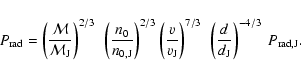
In this section we compare the flux density of different radio sources. Again, to facilitate the comparison, all flux densities in Fig. 4 are normalized to a distance of 1 AU. Note that this is done because for an extrasolar planetary system the star and the planet will have the same distance to a detector at Earth.
![\begin{figure}
{\includegraphics[width=8.8cm,clip]{1976fig4.ps} }\end{figure}](/articles/aa/full/2005/26/aa1976-04/img128.gif) |
Figure 4:
Solar radio data according to Boischot & Denisse (1964) (dotted line) and
Nelson et al. (1985) (solid lines).
Jupiter radio flux during periods of intense activity
(cf. Fig. 2) according to Zarka et al. (2004) (dashed line).
Also shown: quiescent stellar emission from UV Ceti (short-dashed line) and HD 129333
(see Sect. 2.2) and lower limit
for the radio flux expected from |
| Open with DEXTER | |
We first consider the contribution of the galactic background. It is known that the
galactic background depends on the viewing direction. It can be measured by a second
measurement of the sky close to the extrasolar system and then be subtracted from the signal
received from the system. For example, the UTR-2 radio telescope in Kharkov can be used in a two-beam
mode with one of the beams directly on the radio source and the second beam pointing ![]() away from the first beam (Zarka et al. 1997). Another option would be to remove the sky background by
interferometry, see e.g. Nelson et al. (1985).
away from the first beam (Zarka et al. 1997). Another option would be to remove the sky background by
interferometry, see e.g. Nelson et al. (1985).
If Jupiter's radio emissions is compared to the sun's emission, one clearly notes that the planetary emission is far more powerful than the quiet sun emission. Thus the question is not whether an extrasolar planet would be detectable against a sun-like star (during quiet conditions), but rather whether such a quiet star would be detectable against the radiation of such a planet. The slowly varying component (not shown in Fig. 4) does not contribute much to the solar flux in the spectral range where planetary emission is expected.
The quiescent emission some stars exhibit could in principle be problematic.
Although no measurements are available for low frequencies (![]() 1 GHz), it seems likely
that the flux levels are much lower at frequencies relevant for planetary detection (
1 GHz), it seems likely
that the flux levels are much lower at frequencies relevant for planetary detection (![]() 25 MHz).
Also, quiescent radio emission seems to be connected to stellar X-ray emission (Güdel et al. 1995).
Thus, the comparison of the radio emission and the X-ray emission might serve as an indicator of
whether the source of the radio emission is likely to be the star or not. Also, the low degree of
polarization of the quiescent emission (see Sect. 2.2) as opposed to the planetary radio emission will prove to be an important diagnostic tool.
25 MHz).
Also, quiescent radio emission seems to be connected to stellar X-ray emission (Güdel et al. 1995).
Thus, the comparison of the radio emission and the X-ray emission might serve as an indicator of
whether the source of the radio emission is likely to be the star or not. Also, the low degree of
polarization of the quiescent emission (see Sect. 2.2) as opposed to the planetary radio emission will prove to be an important diagnostic tool.
Due to their relatively low occurrence-rate (about 10% of the time near solar maximum, see Sect. 2.1), noise storms are not very important for the case where a Jupiter-like planet is to be detected around a Sun-like star. They could have an influence in systems where either the planetary radio emission is weaker than Jupiter's, or in cases of a star showing more activity than the sun. In these cases statistical considerations would be required, and the quiet star level would have to be evaluated carefully. On the other hand, for close-in extrasolar planets, emission much stronger than Jupiter's is expected. Thus the contribution of noise storms probably is negligible.
Stellar radio bursts are another matter. In the solar system, they are far more powerful than any planetary radio emission. The question arises as to whether the latter could be separated from such a bursty background. Fortunately, these radio bursts do not occur all the time. Although type IV emission can last for several days, it only occurs with a rate of approximately 3 per month during sunspot maximum. Type III emission happens much more frequently (up to 1400 per month at sunspot maximum), but its duration is limited to a few seconds (Boischot & Denisse 1964). Thus it can be hoped that using statistical arguments the stellar bursts can be separated from planetary emission. If one admits the possibility that the beaming direction of extrasolar planetary radio emission could be very different from what we see in the solar system, it could be worth while to look at secondary eclipses of transiting planets as suggested by Richardson et al. (2003). In this case different spectra may be obtained during secondary eclipse ("star only''-spectra when the planet passes behind the star) and off-eclipse ("star plus planet''-spectra). The noisy background of the stellar radio bursts could then be reduced by statistics, i.e. by observing not one but many eclipses of an appropriate planet. Of course, a star with little activity in the radio spectrum (like the Sun near solar minimum) is always preferable.
The planetary radio emission of some extrasolar planets may be much
stronger than Jupiter's emission. For example, for a system similar to
![]() Bootes, the radio emission will be several orders of magnitude stronger than
Jupiter's emission (see Fig. 3). It can be seen that detection is more likely
for young stellar systems, where the stellar wind is denser and faster than for today's Sun. The
radio emission from
Bootes, the radio emission will be several orders of magnitude stronger than
Jupiter's emission (see Fig. 3). It can be seen that detection is more likely
for young stellar systems, where the stellar wind is denser and faster than for today's Sun. The
radio emission from ![]() Bootes at its present age (1.0 Gyr) is much stronger than the
contributions of
the galactic background, the quiet sun emission, solar noise storms, and also the assumed maximum
quiescent radio emission. Some stellar radio bursts will still be more intense than the planetary
emission; depending on the occurrence rate of radio bursts on the star, this might be more or less
problematic. This will be especially true if the planets host star exhibits very strong stellar
flares.
Bootes at its present age (1.0 Gyr) is much stronger than the
contributions of
the galactic background, the quiet sun emission, solar noise storms, and also the assumed maximum
quiescent radio emission. Some stellar radio bursts will still be more intense than the planetary
emission; depending on the occurrence rate of radio bursts on the star, this might be more or less
problematic. This will be especially true if the planets host star exhibits very strong stellar
flares.
Even in cases where the combined stellar/planetary radio signal
contains major contributions from the planet, one also requires some means to separate the two
contributions. There are several ways that this can be achieved. Firstly, it is known that
planetary radio emission is highly polarized (Zarka 1998). This is not the case for the
quiet sun radio emission or the quiescent radio emission (see Sect. 2).
Secondly, the bursty component could possibly be discriminated by occultation during secondary eclipses.
Thirdly, for planets not subjected to tidal locking (i.e. far enough from their star) rotation
rates could help to distinguish the two components. For the solar system it is known that the
radio emissions are modulated with the planetary rotation, which is of the order of hours,
whereas the stellar rotation is measured in days. This method will fail in the few cases where
the stellar and the planetary rotation are synchronized. As discussed by Pätzold & Rauer (2002),
some measurements of the stellar rotation period of ![]() Bootes seem to indicate that this is
the case (this is also suggested by Leigh et al. 2003), while other values suggest that the star is rotating more slowly. But even if the
method is not applicable to
Bootes seem to indicate that this is
the case (this is also suggested by Leigh et al. 2003), while other values suggest that the star is rotating more slowly. But even if the
method is not applicable to ![]() Bootes, the modulation with the rotation period may be very
useful for other stellar systems.
Bootes, the modulation with the rotation period may be very
useful for other stellar systems.
We have compared the radio flux expected from close-in giant extrasolar planets with the
different radiation components of their host stars.
For this purpose, a planetary radio scaling calibrated by the radio spectrum of Jupiter obtained
from recent Cassini data
(Zarka et al. 2004) was presented.
Care must be taken not to produce unphysical results: The condition
![]() always
should be checked.
Several extrasolar planets were discussed; it was shown that due
to tidal locking, many of the close-in planets (
always
should be checked.
Several extrasolar planets were discussed; it was shown that due
to tidal locking, many of the close-in planets (![]() AU) are only weakly magnetized,
leading to a maximum frequency below the ionospheric cutoff limit. Other planets have a stronger
magnetic moment (either because of their even smaller orbital radius, like OGLE-TR-113 b, or due
to their larger mass, like
AU) are only weakly magnetized,
leading to a maximum frequency below the ionospheric cutoff limit. Other planets have a stronger
magnetic moment (either because of their even smaller orbital radius, like OGLE-TR-113 b, or due
to their larger mass, like ![]() Bootes). For these planets, detection is possible in principle,
provided the planet is not located too far away from the Earth (which is the case for OGLE-TR-113
b).
On the other hand, similar planets may well exist closer to Earth.
It was also shown that because of the stellar wind evolution, the radio flux from young
systems is much more important.
Thus, the best candidates for planetary radio detection seem to be young,
massive "Hot Jupiters'' not too far away from the Earth.
It was shown that at least for one system (
Bootes). For these planets, detection is possible in principle,
provided the planet is not located too far away from the Earth (which is the case for OGLE-TR-113
b).
On the other hand, similar planets may well exist closer to Earth.
It was also shown that because of the stellar wind evolution, the radio flux from young
systems is much more important.
Thus, the best candidates for planetary radio detection seem to be young,
massive "Hot Jupiters'' not too far away from the Earth.
It was shown that at least for one system (![]() Bootes), intense radio emission is expected,
which should in principle be detectable on Earth with the next generation of radio telescopes
(LOFAR), and maybe even before that.
Past observations like those of Zarka et al. (1997) and Bastian et al. (2000) were either not sensitive
enough or were limited to higher frequencies.
Note that a space-based radio observatory would avoid the restriction of the frequency range
caused by the ionospheric cutoff.
Bootes), intense radio emission is expected,
which should in principle be detectable on Earth with the next generation of radio telescopes
(LOFAR), and maybe even before that.
Past observations like those of Zarka et al. (1997) and Bastian et al. (2000) were either not sensitive
enough or were limited to higher frequencies.
Note that a space-based radio observatory would avoid the restriction of the frequency range
caused by the ionospheric cutoff.
Different methods were presented which might prove useful for the discrimination of the different
contributions of star and planet to the total radio signal.
It was shown that for the ![]() Bootes system, the contribution of the planetary radio signal
will dominate over the stellar radio flux, except for strong radio bursts. If the star's radio
bursts are comparable to solar radio bursts, it should be possible to extract the planetary radio
characteristics from the combined stellar and planetary signal.
Bootes system, the contribution of the planetary radio signal
will dominate over the stellar radio flux, except for strong radio bursts. If the star's radio
bursts are comparable to solar radio bursts, it should be possible to extract the planetary radio
characteristics from the combined stellar and planetary signal.
This comparison shows that radio observations of an extrasolar planetary systems will yield information not only on the stellar emission, but also on the planetary radio emission in the near future.
Acknowledgements
We would like to thank the referee for comments and suggestions. J.-M.G. thanks A. Benz for additional comments. This research has made use of the VizieR catalogue access tool, CDS, Strasbourg, France.