A&A 434, 827-838 (2005)
DOI: 10.1051/0004-6361:20041827
S. A. Levshakov1 - M. Centurión2 - P. Molaro2 - S. D'Odorico3
1 - Department of Theoretical Astrophysics,
Ioffe Physico-Technical Institute, 194021 St. Petersburg, Russia
2 -
Osservatorio Astronomico di Trieste, via G. B. Tiepolo 11,
34131 Trieste, Italy
3 -
European Southern Observatory, Karl-Schwarzschild-Strasse 2,
85748 Garching bei München, Germany
Received 10 August 2004 / Accepted 12 January 2005
Abstract
We propose a new methodology for probing the cosmological
variability of ![]() from pairs of Fe II lines (SIDAM, single ion differential
from pairs of Fe II lines (SIDAM, single ion differential ![]() measurement) observed in individual exposures from a high resolution spectrograph.
By this we avoid the influence of the spectral shifts due to
(i) ionization inhomogeneities in the absorbers; and (ii) non-zero offsets between different exposures. Applied to the Fe II lines of the metal absorption line system at
measurement) observed in individual exposures from a high resolution spectrograph.
By this we avoid the influence of the spectral shifts due to
(i) ionization inhomogeneities in the absorbers; and (ii) non-zero offsets between different exposures. Applied to the Fe II lines of the metal absorption line system at
![]() = 1.839 in the spectrum of Q 1101-264 obtained by means of
the UV-Visual Echelle Spectrograph (UVES) at the ESO Very Large Telescope (VLT),
SIDAM provides
= 1.839 in the spectrum of Q 1101-264 obtained by means of
the UV-Visual Echelle Spectrograph (UVES) at the ESO Very Large Telescope (VLT),
SIDAM provides
![]() =
=
![]() .
The
.
The
![]() = 1.15 Fe II system toward HE 0515-4414
has been re-analyzed by this method thus obtaining for the combined sample
= 1.15 Fe II system toward HE 0515-4414
has been re-analyzed by this method thus obtaining for the combined sample
![]() =
=
![]() .
These values are shifted with respect to the Keck/HIRES mean
.
These values are shifted with respect to the Keck/HIRES mean
![]() =
=
![]() (Murphy et al. 2004) at very high confidence level (95%).
The fundamental photon noise limitation in the
(Murphy et al. 2004) at very high confidence level (95%).
The fundamental photon noise limitation in the
![]() measurement with the VLT/UVES is discussed
to figure the prospects for future observations. It is suggested that with a spectrograph of
measurement with the VLT/UVES is discussed
to figure the prospects for future observations. It is suggested that with a spectrograph of
![]() 10 times the UVES dispersion coupled to a 100 m class telescope
the present Oklo level (
10 times the UVES dispersion coupled to a 100 m class telescope
the present Oklo level (
![]()
![]() 4.5
4.5 ![]() 10-8) can be achieved
along cosmological distances with differential measurements of
10-8) can be achieved
along cosmological distances with differential measurements of
![]() .
.
Key words: cosmology: observations - line: profiles - galaxies: quasars: absorption lines - galaxies: quasars: individual: Q 1101-264, HE 0515-4414
The variability of the fundamental physical constants over cosmic time, firstly proposed almost seven decades ago (Milne 1937; Dirac 1937), has been subsequently investigated in various aspects by many authors (for a review see, e.g., Uzan 2003).
The Sommerfeld fine-structure constant,
![]() ,
which describes
electromagnetic and optical properties of atoms, is the most suitable
for time variation tests in both laboratory experiments with atomic clocks and
astronomical observations. The value of this constant is known with
high accuracy,
,
which describes
electromagnetic and optical properties of atoms, is the most suitable
for time variation tests in both laboratory experiments with atomic clocks and
astronomical observations. The value of this constant is known with
high accuracy,
![]() (Mohr & Tailor 2000), and its
time- dependence is restricted in the laboratory experiments at
the level of dln
(Mohr & Tailor 2000), and its
time- dependence is restricted in the laboratory experiments at
the level of dln
![]() yr-1,
corresponding to an upper limit of
yr-1,
corresponding to an upper limit of
![]() yr-1(Fischer et al. 2004). At the cosmological time-scale
yr-1(Fischer et al. 2004). At the cosmological time-scale
![]() yr (z > 1), this limit transforms into
yr (z > 1), this limit transforms into
![]() ,
if
,
if ![]() ,
the value of
,
the value of ![]() at redshift z, is a linear function of t.
The functional dependence of the gauge-coupling constants on t is, however, unknown and theory predicts even oscillations during the course of the cosmological evolution (e.g., Marciano 1984). In this regard the astronomical observations are the only way
to test such predictions at different space-time coordinates (see, e.g.,
Mota & Barrow 2004, where the effects of inhomogeneous space and time evolution
of
at redshift z, is a linear function of t.
The functional dependence of the gauge-coupling constants on t is, however, unknown and theory predicts even oscillations during the course of the cosmological evolution (e.g., Marciano 1984). In this regard the astronomical observations are the only way
to test such predictions at different space-time coordinates (see, e.g.,
Mota & Barrow 2004, where the effects of inhomogeneous space and time evolution
of ![]() are studied).
are studied).
The astronomical measurements of the fine-structure splittings
of emission lines in distant galaxies started by Savedoff (1956)
are summarized in a recent comprehensive work by
Bahcall et al. (2004, hereafter BSS):
![]() in the
range
0.16 < z < 0.80
in the
range
0.16 < z < 0.80![]() . The most stringent bound in the overlapping interval
. The most stringent bound in the overlapping interval
![]() ,
stemming from the radioactive decay rates of certain long-lived nuclei
found in meteoritic data, is set by Olive et al. (2004):
,
stemming from the radioactive decay rates of certain long-lived nuclei
found in meteoritic data, is set by Olive et al. (2004):
![]() .
The time interval comparable with the meteoritic analysis is covered by
the Oklo natural reactor (
.
The time interval comparable with the meteoritic analysis is covered by
the Oklo natural reactor (
![]() yr).
Recent reanalysis of the isotopic abundances in the samples taken from Oklo
provides an intriguing result that the value of
yr).
Recent reanalysis of the isotopic abundances in the samples taken from Oklo
provides an intriguing result that the value of ![]() was larger in the past:
was larger in the past:
![]()
![]() (Lamoreaux & Torgerson 2004).
(Lamoreaux & Torgerson 2004).
At higher redshifts the variability of ![]() can be tested by
observations of small shifts between different ionic transitions in the
absorption-line spectra of quasars (Bahcall et al. 1967).
This technique, now known as the alkali doublet (AD) method,
was utilized in numerous studies (for a review, see BSS).
The best constraint obtained by the AD method is
can be tested by
observations of small shifts between different ionic transitions in the
absorption-line spectra of quasars (Bahcall et al. 1967).
This technique, now known as the alkali doublet (AD) method,
was utilized in numerous studies (for a review, see BSS).
The best constraint obtained by the AD method is
![]() (Murphy et al. 2001).
(Murphy et al. 2001).
The AD method was generalized by Webb et al. (1999)
and Dzuba et al. (1999, 2002)
in the many-multiplet (MM) method which provides an order
of magnitude improvement in the accuracy of the estimations of
![]() .
Being applied to 143 metal absorption systems (the dominant ions Mg II, Fe II
at z < 1.8, and Al II, Si II at z > 1.8)
identified in the Keck/HIRES spectra of quasars, the MM method indicates, opposite to the recent Oklo result, a decrease of
.
Being applied to 143 metal absorption systems (the dominant ions Mg II, Fe II
at z < 1.8, and Al II, Si II at z > 1.8)
identified in the Keck/HIRES spectra of quasars, the MM method indicates, opposite to the recent Oklo result, a decrease of ![]() with cosmic time:
with cosmic time:
![]() in the redshift range
0.2 < z < 4.2 (Murphy et al. 2004, hereafter MFWDPW).
in the redshift range
0.2 < z < 4.2 (Murphy et al. 2004, hereafter MFWDPW).
A potential concern is that this result includes some systematics. Indeed, an increasing accuracy of the
![]() measurements requires a careful consideration of
the intrinsic structure of the atomic transitions which is formed by
the isotope shifts and hyperfine splittings (Levshakov 1994).
For instance, the error of the mean
measurements requires a careful consideration of
the intrinsic structure of the atomic transitions which is formed by
the isotope shifts and hyperfine splittings (Levshakov 1994).
For instance, the error of the mean
![]() corresponds to the error of the line center of
corresponds to the error of the line center of ![]() 20 m s-1 (see Eq. (12) in Levshakov 2004, hereafter L04) which is about 40 times smaller than the isotope shift
between 26,24Mg II transitions
20 m s-1 (see Eq. (12) in Levshakov 2004, hereafter L04) which is about 40 times smaller than the isotope shift
between 26,24Mg II transitions
![]() ,
,
![]() m s-1 (Drullinger et al. 1980). Unfortunately, the influence of the isotope shifts cannot be well specified since we do not know the isotope abundances at different redshifts.
If the isotope abundance ratio indeed varies with z,
the isotope shifts may imitate the non-zero
m s-1 (Drullinger et al. 1980). Unfortunately, the influence of the isotope shifts cannot be well specified since we do not know the isotope abundances at different redshifts.
If the isotope abundance ratio indeed varies with z,
the isotope shifts may imitate the non-zero
![]() value
(Ashenfelter et al. 2004; Kozlov et al. 2004, hereafter KKBDF).
On the other hand, at metallicities of
value
(Ashenfelter et al. 2004; Kozlov et al. 2004, hereafter KKBDF).
On the other hand, at metallicities of
![]() , - typical for the QSO systems
with low ions, - the isotope abundances may not differ considerably from terrestrial (Murphy et al. 2003; Chand et al. 2004, hereafter CSPA).
, - typical for the QSO systems
with low ions, - the isotope abundances may not differ considerably from terrestrial (Murphy et al. 2003; Chand et al. 2004, hereafter CSPA).
The influence of unknown isotopic ratio and of another source of systematics caused by
inhomogeneous ionization structure within the absorber can be considerably
diminished if only one heavy element like, e.g., Fe II,
is used in the
![]() measurement (L04). In spite of a rather low present accuracy of the theoretical calculations of the isotope shift parameters for atoms with more than one valence
electron (
measurement (L04). In spite of a rather low present accuracy of the theoretical calculations of the isotope shift parameters for atoms with more than one valence
electron (![]() 50%, KKBDF), the isotopic effect for Fe II (seven valence electrons in the configuration
50%, KKBDF), the isotopic effect for Fe II (seven valence electrons in the configuration
![]() )
is less pronounced than that
for Mg II (one valence electron in the configuration
)
is less pronounced than that
for Mg II (one valence electron in the configuration ![]() )
for two reasons:
(i) iron is heavier and its isotope structure is more compact;
and (ii) the relative abundance of the leading isotope 56Fe is higher
)
for two reasons:
(i) iron is heavier and its isotope structure is more compact;
and (ii) the relative abundance of the leading isotope 56Fe is higher![]() . Therefore systematic shifts in
. Therefore systematic shifts in
![]() due to unknown isotopic compositions should be smaller in the analysis of the Fe II data.
due to unknown isotopic compositions should be smaller in the analysis of the Fe II data.
This approach applied to the Fe II system identified
at
![]() = 1.15 in the VLT/UVES spectrum of the bright quasar HE 0515-4414 (B = 15.0) gave
= 1.15 in the VLT/UVES spectrum of the bright quasar HE 0515-4414 (B = 15.0) gave
![]() (Quast et al. 2004, hereafter QRL).
(Quast et al. 2004, hereafter QRL).
The most stringent limit on the variability of ![]() ,
,
![]() ,
standard deviation
,
standard deviation
![]() ,
was claimed by CSPA. Their result is based on the VLT/UVES observations of 23 absorption systems
(
,
was claimed by CSPA. Their result is based on the VLT/UVES observations of 23 absorption systems
(
![]() )
toward 18 QSOs. In this study, the MM method was applied to
a more homogeneous ensemble of Mg II, Si II, and Fe II lines which are not strongly saturated and show a less complex structure as compared with the metal profiles from MFWDPW.
)
toward 18 QSOs. In this study, the MM method was applied to
a more homogeneous ensemble of Mg II, Si II, and Fe II lines which are not strongly saturated and show a less complex structure as compared with the metal profiles from MFWDPW.
It should be noted, however, that the measurements with dispersions
![]() (
(
![]() m s-1)
are already at the sensitivity limit of the UVES and, hence, they
may be affected by the data reduction procedure and/or by
the changing in time characteristics of the device itself.
There are three main sources of potential systematic errors in the absolute velocity scale:
(i) temperature; and (ii) air pressure instability; and (iii) mechanical instabilities of unknown origin. For instance, a change of 1 millibar (or a change of 0.3
m s-1)
are already at the sensitivity limit of the UVES and, hence, they
may be affected by the data reduction procedure and/or by
the changing in time characteristics of the device itself.
There are three main sources of potential systematic errors in the absolute velocity scale:
(i) temperature; and (ii) air pressure instability; and (iii) mechanical instabilities of unknown origin. For instance, a change of 1 millibar (or a change of 0.3 ![]() C) induces an error in radial velocities of
C) induces an error in radial velocities of ![]() 50 m s-1 (Kaufer et al. 2004).
50 m s-1 (Kaufer et al. 2004).
In the present paper we investigate step by step the data reduction procedure usually applied to the VLT/UVES spectra in order to reveal possible systematics and to design the optimal measurement technique to avoid them. The analysis is based on another Fe II system identified in the absorption-line spectrum of quasar Q 1101-264.
The paper is organized as follows. In Sect. 2 we describe observations and data
reduction performed to construct our Fe II sample. Small velocity shifts
(equivalent to 0.1-0.2 pixel size) between the scientific exposures are
analyzed in Sect. 3. Being ignored, such shifts may affect the shapes of the
Fe II profiles in the co-added spectra, leading to their inconsistency.
Section 4 presents the key procedure used to study the time dependence of ![]() ,
including error estimation. The results of our analysis are explained in Sect. 5.
Section 6 gives the fundamental noise limitation in the
,
including error estimation. The results of our analysis are explained in Sect. 5.
Section 6 gives the fundamental noise limitation in the
![]() measurement due to
photon count and spectral profile. The quality factor similar to that introduced
by Connes (1985) to optimize measurements of the stellar radial velocities is
defined and calculated in this section.
It can be used to control the sample dispersion in
measurement due to
photon count and spectral profile. The quality factor similar to that introduced
by Connes (1985) to optimize measurements of the stellar radial velocities is
defined and calculated in this section.
It can be used to control the sample dispersion in
![]() .
The obtained results and future prospects are discussed in Sect. 7. Our conclusions
are given in Sect. 8.
.
The obtained results and future prospects are discussed in Sect. 7. Our conclusions
are given in Sect. 8.
Table 1: ESO UVES archive data on the quasar Q 1101-264.
The most accurate measurements of
![]() can be
carried out with unsaturated Fe II lines which lie outside
the Ly-
can be
carried out with unsaturated Fe II lines which lie outside
the Ly-![]() forest and are not corrupted by any other absorption and/or
telluric lines. The components of the Fe II lines should be
clearly distinguished. Besides, a QSO should be a bright object to provide a
high S/N ratio. These requirements are fulfilled for the
forest and are not corrupted by any other absorption and/or
telluric lines. The components of the Fe II lines should be
clearly distinguished. Besides, a QSO should be a bright object to provide a
high S/N ratio. These requirements are fulfilled for the
![]() = 1.839 system toward
Q 1101-264 with
= 1.839 system toward
Q 1101-264 with
![]() = 2.145 and V = 16.02, which was discovered by
Osmer & Smith (1977). The absorption system was identified by
Carswell et al. (1982) and investigated with high spectral resolution by
Petitjean et al. (2000) and Dessauges-Zavadsky et al. (2003)
who used the same UVES/VLT data as in the present work. This system was also studied with lower resolution in a series of works by Boksenberg & Snijders (1981),
Young et al. (1982), Carswell et al. (1984),
and Lanzetta et al. (1987).
= 2.145 and V = 16.02, which was discovered by
Osmer & Smith (1977). The absorption system was identified by
Carswell et al. (1982) and investigated with high spectral resolution by
Petitjean et al. (2000) and Dessauges-Zavadsky et al. (2003)
who used the same UVES/VLT data as in the present work. This system was also studied with lower resolution in a series of works by Boksenberg & Snijders (1981),
Young et al. (1982), Carswell et al. (1984),
and Lanzetta et al. (1987).
The observations were acquired with the UVES at
the VLT 8.2 m telescope at Paranal, Chile, and the spectral data were
retrieved from the ESO archive. The high resolution spectra
of Q 1101-264 were obtained during the UVES Science Verification programme
for the study of the Ly-![]() forest (Kim et al. 2002).
The spectra used here were recorded with a dichroic filter which allows
to work with the blue and red UVES arms simultaneously as with two independent spectrographs.
The standard settings with central wavelengths at
forest (Kim et al. 2002).
The spectra used here were recorded with a dichroic filter which allows
to work with the blue and red UVES arms simultaneously as with two independent spectrographs.
The standard settings with central wavelengths at ![]() 437 nm and
437 nm and ![]() 860 nm
were used for the blue and red arms, respectively. From the blue spectra we used only order 102, and from the red spectra - orders 90 and 83, where Fe II lines suitable for the
860 nm
were used for the blue and red arms, respectively. From the blue spectra we used only order 102, and from the red spectra - orders 90 and 83, where Fe II lines suitable for the
![]() measurement are observed. Details of the observations are presented in Table 1.
Columns 1 and 2 give the exposure archive number and the setting used. Columns 3-7 list the QSO data, and Cols. 8-11 the data of the closest in time calibration thorium-argon (ThAr) lamp.
measurement are observed. Details of the observations are presented in Table 1.
Columns 1 and 2 give the exposure archive number and the setting used. Columns 3-7 list the QSO data, and Cols. 8-11 the data of the closest in time calibration thorium-argon (ThAr) lamp.
In this work we analyze five exposures (No. 5/6, 11/12, 19/20, 21/22, and 23/24)
of 3600 s obtained over four nights in February 2000 with seeing as indicated in Col. 5 of Table 1. The slit widths were both set at 0.8 arcsec and the CCDs were read-out in 1 ![]() 2 binned pixels (spatial
2 binned pixels (spatial ![]() dispersion direction).
The resulting spectral resolution as measured from the ThAr emission lines is of
FWHM
dispersion direction).
The resulting spectral resolution as measured from the ThAr emission lines is of
FWHM ![]() 6.0 km s-1 in the blue (
6.0 km s-1 in the blue (
![]() Å),
and of
Å),
and of ![]() 5.4 km s-1 in the red (
5.4 km s-1 in the red (
![]() Å)
Å)
We used the UVES pipeline (the routines implemented in MIDAS-ESO data
reduction package for UVES data) to perform the bias correction, inter-order background subtraction,
flat-fielding, correction of cosmic rays impacts, sky subtraction, extraction of the orders in the pixel space and wavelength calibration. A modified version of the routine "echred'' of the context ECHELLE inside MIDAS was used to calibrate in wavelength the echelle spectra without rebinning.
In this way we have the reduced spectra with their original pixel size in
wavelength. This corresponds to a sampling of 50 mÅ (3.3 km s-1/pix) for the blue and
55 mÅ (2.2 km s-1/pix) for the red. Typical rms of the wavelength calibration is less than one-fiftieth of a pixel, or
![]() mÅ (
mÅ (![]() 60 m s-1).
The observed wavelength scale of each spectrum was transformed into vacuum,
heliocentric wavelength scale (Edlén 1966).
At first stage of our analysis we followed the standard procedure and added together
the single extracted spectra using weights proportional to the square of their S/N.
Before being added, the spectra were re-sampled to an equidistant wavelength grid
(50 mÅ/pix) using linear interpolation.
60 m s-1).
The observed wavelength scale of each spectrum was transformed into vacuum,
heliocentric wavelength scale (Edlén 1966).
At first stage of our analysis we followed the standard procedure and added together
the single extracted spectra using weights proportional to the square of their S/N.
Before being added, the spectra were re-sampled to an equidistant wavelength grid
(50 mÅ/pix) using linear interpolation.
The Fe II profiles in the
![]() = 1.8389 systems toward Q 1101-264
consist of at least 6 subcomponents spread over 100 km s-1 (Dessauges-Zavadsky
et al. 2003). The central component, seen in all but one Fe II lines from Table 2 (the undetected
= 1.8389 systems toward Q 1101-264
consist of at least 6 subcomponents spread over 100 km s-1 (Dessauges-Zavadsky
et al. 2003). The central component, seen in all but one Fe II lines from Table 2 (the undetected
![]() Å has the smallest
oscillator strength), is marginally blended in the blue wing with
weak component at v = -17.6 km s-1 (see Fig. 1). Henceforth we will use this central component in the
Å has the smallest
oscillator strength), is marginally blended in the blue wing with
weak component at v = -17.6 km s-1 (see Fig. 1). Henceforth we will use this central component in the
![]() measurement.
measurement.
Table 2:
Atomic data of the Fe II transitionsa, the sensitivity coefficients
![]() ,
and the isotope mass shift constants
,
and the isotope mass shift constants
![]() c. Estimated errors are given in parentheses.
c. Estimated errors are given in parentheses.
![\begin{figure}
\par\includegraphics[height=7.2cm,width=17.35cm,clip]{1827fig1.ps}\end{figure}](/articles/aa/full/2005/18/aa1827/img66.gif) |
Figure 1:
Combined absorption-line spectra of Fe II associated with the
|
| Open with DEXTER | |
We carefully checked that the profiles shown in Fig. 1 are free from cosmic rays and telluric absorptions. The combined spectra reveal high signal-to-noise ratios, 100 ![]() S/N
S/N ![]() 160. The continuum levels are very well defined for all iron lines since in all
cases there are large "continuum windows'' at both sides of each
Fe II absorption. But, nevertheless, we failed to find a model which could adequately describe the stacked profiles. Using the multicomponent Voigt profile fitting procedure
we obtained the best normalized
160. The continuum levels are very well defined for all iron lines since in all
cases there are large "continuum windows'' at both sides of each
Fe II absorption. But, nevertheless, we failed to find a model which could adequately describe the stacked profiles. Using the multicomponent Voigt profile fitting procedure
we obtained the best normalized
![]() for the number of degrees of freedom
for the number of degrees of freedom ![]() .
The source of such high
.
The source of such high
![]() value is clearly seen in Fig. 1:
some portions of the Fe II profiles are not in concordance with each other.
value is clearly seen in Fig. 1:
some portions of the Fe II profiles are not in concordance with each other.
This inconsistency in the combined Fe II spectra may reflect some hidden problems in the standard data reduction procedure. We investigate this question in the next section.
In order to understand the origin of the discrepancy between Fe II profiles,
we firstly investigated distortion and wavelength calibration.
It turned out that two Fe II lines
![]() and
and
![]() lie close to the starting and end points of the echelle orders where distortions in the spectral sensitivity
are the largest. These lines were excluded from the further analysis.
The remaining Fe II lines are observed in the central parts of the echelle orders.
lie close to the starting and end points of the echelle orders where distortions in the spectral sensitivity
are the largest. These lines were excluded from the further analysis.
The remaining Fe II lines are observed in the central parts of the echelle orders.
Then we selected isolated and unblended ThAr lines from these central spectral
regions and compared their profiles. The time intervals between
calibration exposures are large and the ThAr spectra were taken under different
conditions. Namely, the differences between the mean temperatures and air pressures
are
![]() C,
C,
![]() C, and
C, and
![]() mb,
mb,
![]() mb, respectively (see Table 1).
Changes in T and P lead to the velocity shifts between exposures. For instance, emission profiles plotted in Fig. 2 show that in the blue arm
mb, respectively (see Table 1).
Changes in T and P lead to the velocity shifts between exposures. For instance, emission profiles plotted in Fig. 2 show that in the blue arm
![]() mÅ (
mÅ (
![]() m s-1)
and
m s-1)
and
![]() mÅ (
mÅ (
![]() m s-1),
whereas in the red arm
m s-1),
whereas in the red arm
![]() equals
equals
![]() ,
as expected, but
,
as expected, but
![]() mÅ (
mÅ (
![]() m s-1) which
is 1.6 times larger than
m s-1) which
is 1.6 times larger than
![]() (exposures 11 and 12 are taken
for references). If the velocity drifts were entirely due to temperature and pressure changes, then we would observe a monotonous shift identical in the blue and red arms, as in the case of the 21st and 22nd exposures. The deviation from this behavior revealed for the 5th and 6th exposures indicates that the third factor - some mechanical instabilities - may also be important. Since it is impossible to control what kind of distortions are caused by mechanical instabilities, we remove the scientific exposures 5 and 6 from the study.
(exposures 11 and 12 are taken
for references). If the velocity drifts were entirely due to temperature and pressure changes, then we would observe a monotonous shift identical in the blue and red arms, as in the case of the 21st and 22nd exposures. The deviation from this behavior revealed for the 5th and 6th exposures indicates that the third factor - some mechanical instabilities - may also be important. Since it is impossible to control what kind of distortions are caused by mechanical instabilities, we remove the scientific exposures 5 and 6 from the study.
![\begin{figure}
\par\includegraphics[height=14.5cm,width=7.6cm,clip]{1827fig2.ps}\end{figure}](/articles/aa/full/2005/18/aa1827/img85.gif) |
Figure 2: Emission line profiles from the thorium-argon calibration lamp. The lines are placed close to the centers of the UVES echelle orders of different settings which are indicated at the top left hand corners in the panels. The wavelength step size corresponds to the original pixel width. The numbering of the histograms are in accord with the list in Table 1. The 11th and 12th exposures are taken as reference. Note the difference between the relative shifts 5-11 and 6-12, while 21-11 and 22-12 show identical velocity offsets. |
| Open with DEXTER | |
This analysis shows that in order to avoid uncertainties in the wavelength calibration caused by changes in temperature and/or pressure, the calibration ThAr lamps must be taken just before and after the scientific exposure. If for some exposures the relative shifts of the ThAr lines in the blue and red arms turn out to be different, these exposures must be excluded from the consideration since they are influenced by mechanical instabilities which cannot be properly corrected.
Following the standard reduction procedure the remaining scientific exposures
should be co-added to enhance S/N. However, this step can introduce additional
uncertainties because every calibrated exposure has its own velocity offset.
Note that the combination of the exposures
by means of the MIDAS package requires the same starting wavelength,
number of points, and the step size. Such procedure cancels out the original non-zero
offsets between the individual exposures and smears out small shifts.
This can perturb the line centroids, especially those of narrow absorption
lines with sharp intensity gradients.
Since in the
![]() measurement the accuracy of the line position is the key factor,
it is more appropriate to work with individual exposures which have lower S/N rather
than with a high S/N combined spectrum.
measurement the accuracy of the line position is the key factor,
it is more appropriate to work with individual exposures which have lower S/N rather
than with a high S/N combined spectrum.
Accounting for these arguments we selected the scientific exposures with
Fe II lines shown in Fig. 3. All spectra are vacuum and heliocentric
calibrated with only one ThAr spectrum (exposures 11 and 12 for the blue and
red frames, respectively), they are not combined and not resampled.
The unknown velocity offsets arising from such calibration
are canceled out in the differential measurements of
![]() as
described in the next section.
as
described in the next section.
The key line in our approach is Fe II
![]() since its sensitivity
coefficient is negative, while the other iron transitions
have positive
since its sensitivity
coefficient is negative, while the other iron transitions
have positive ![]() -values (Table 2). A relatively low
strength of the
-values (Table 2). A relatively low
strength of the
![]() line requires S/N
line requires S/N ![]() 30 in individual exposures
in order to measure its center accurately. This requirement is fulfilled for
Q 1101-264 (see Fig. 4, where the S/N values are indicated).
It is also important that for this system the accuracy of the
normalization of the Fe II profiles leaves no room for doubts since the local
continua (the horizontal lines in Fig. 3) are calculated with high precision.
In each panel in Fig. 3, dots with error bars indicate the mean
intensities and their 1
30 in individual exposures
in order to measure its center accurately. This requirement is fulfilled for
Q 1101-264 (see Fig. 4, where the S/N values are indicated).
It is also important that for this system the accuracy of the
normalization of the Fe II profiles leaves no room for doubts since the local
continua (the horizontal lines in Fig. 3) are calculated with high precision.
In each panel in Fig. 3, dots with error bars indicate the mean
intensities and their 1![]() uncertainties utilized in the
linear regression analysis applied to determine the local continuum level. The uncertainty of the calculated continuum is found to be less than 1% for all selected Fe II spectra.
uncertainties utilized in the
linear regression analysis applied to determine the local continuum level. The uncertainty of the calculated continuum is found to be less than 1% for all selected Fe II spectra.
![\begin{figure}
\par\includegraphics[height=15cm,width=15cm,clip]{1827fig3.ps}\end{figure}](/articles/aa/full/2005/18/aa1827/img89.gif) |
Figure 3:
Unnormalized portions of the Q 1101-264 spectra with the Fe II lines (
|
| Open with DEXTER | |
The standard many-multilet (MM) technique (Webb et al. 1999;
Dzuba et al. 1999, 2002) calculates
![]() using a quite complex procedure.
This leads to potential systematic uncertainties
which may affect both the line profile and the origin of the wavelength scale.
The systematic effects are thoroughly discussed in
Murphy et al. (2003), BSS, and L04. In this section we describe how to
use a modified MM procedure to calculate
using a quite complex procedure.
This leads to potential systematic uncertainties
which may affect both the line profile and the origin of the wavelength scale.
The systematic effects are thoroughly discussed in
Murphy et al. (2003), BSS, and L04. In this section we describe how to
use a modified MM procedure to calculate
![]() directly from the
differences between the wavelengths of a pair of Fe II transitions
observed in the individual exposures. Thereafter this approach is called
a "single ion differential
directly from the
differences between the wavelengths of a pair of Fe II transitions
observed in the individual exposures. Thereafter this approach is called
a "single ion differential ![]() measurement'' (SIDAM).
An important point is that being applied to the lines from the same
exposure, this method does not depend on the unknown offsets of the wavelength scale.
measurement'' (SIDAM).
An important point is that being applied to the lines from the same
exposure, this method does not depend on the unknown offsets of the wavelength scale.
The MM method utilizes the fact that the energy of each line
transitions depends individually on a change in ![]() .
Namely,
the frequency of each transition has its own relativistic correction
to the changes in
.
Namely,
the frequency of each transition has its own relativistic correction
to the changes in ![]() which is expressed by the coefficient q (Dzuba et al. 1999, 2002). Then, the systemic rest wavenumber
which is expressed by the coefficient q (Dzuba et al. 1999, 2002). Then, the systemic rest wavenumber
![]() is given by
is given by
In fact, this approach is similar to the method developed by
Varshalovich & Levshakov (1993) in order to infer the cosmological
variability of the proton-electron mass ratio,
![]() ,
from the analysis of molecular hydrogen H2 absorption lines.
The dependence of the frequencies of electron-vibro-rotational
transitions on a change in
,
from the analysis of molecular hydrogen H2 absorption lines.
The dependence of the frequencies of electron-vibro-rotational
transitions on a change in ![]() differs for individual transitions and
can be characterized by the dimensionless sensitivity coefficient
differs for individual transitions and
can be characterized by the dimensionless sensitivity coefficient ![]() .
The estimation of
.
The estimation of
![]() can be obtained from linear
regression analysis of the
can be obtained from linear
regression analysis of the
![]() pairs from a sample of the
H2 lines (Potekhin et al. 1998; Levshakov et al. 2002b).
Below this technique is applied to the
pairs from a sample of the
H2 lines (Potekhin et al. 1998; Levshakov et al. 2002b).
Below this technique is applied to the
![]() measurement.
measurement.
We can re-write (1) in linear approximation (
![]() )
in the form (L04):
)
in the form (L04):
In this approach, the value of
![]() can be directly estimated from a pair of lines with different sensitivity coefficients. It is easy to show that
can be directly estimated from a pair of lines with different sensitivity coefficients. It is easy to show that
The computational procedure can be slightly modified if we use another variables similar to those introduced in the AD analysis by BSS.
Let us consider an absorption line system at redshift z where a set of
Fe II transitions is formed at the corresponding cosmic time t.
Then, the ratio of the observed wavelengths
![]() to (1+z) defines
the rest wavelengths
to (1+z) defines
the rest wavelengths
![]() which may differ from their present-day
values
which may differ from their present-day
values
![]() ,
if
,
if
![]() .
From (1) one obtains in linear approximation
.
From (1) one obtains in linear approximation
![\begin{figure}
\par\includegraphics[height=17.3cm,width=17.5cm,clip]{1827fig4.ps}\end{figure}](/articles/aa/full/2005/18/aa1827/img119.gif) |
Figure 4:
Individual exposures of the Fe II lines in the spectrum
of Q 1101-264 (normalized intensities are shown by
dots with 1 |
| Open with DEXTER | |
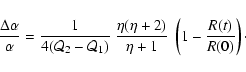
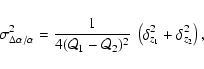
In this section we calculate the uncertainty on individual
![]() measurement caused by the errors in the wavelengths.
The standard method of error propagation is used.
measurement caused by the errors in the wavelengths.
The standard method of error propagation is used.
From Eq. (4) we deduce (taking into account
![]() )
)
We note that the best precision reached today in the measurements of
stellar radial velocities of relatively bright stars is a few m s-1.
Observations with HARPS provide, for example, the rms uncertainty of
2 m s-1 (Pepe et al. 2004) which is close to the HARPS fundamental noise limitation.
For the
![]() measurement with UVES, the fundamental noise
limitation due to spectral profile and photon count is considered in Sect. 6.
measurement with UVES, the fundamental noise
limitation due to spectral profile and photon count is considered in Sect. 6.
The
![]() measurement on the scale of
measurement on the scale of ![]()
![]() can be affected by the isotopic shifts if the ratio
can be affected by the isotopic shifts if the ratio
![]() Fe/56Fe varies between the absorbers (the influence of the isotope 57Fe is negligible because of its relatively low abundance).
Following KKBDF and using their mass shift constants
Fe/56Fe varies between the absorbers (the influence of the isotope 57Fe is negligible because of its relatively low abundance).
Following KKBDF and using their mass shift constants
![]() for Fe II transitions (Table 2), we can estimate the shift of the line center of gravity
mimicking a non-zero
for Fe II transitions (Table 2), we can estimate the shift of the line center of gravity
mimicking a non-zero
![]() :
:
Numerical simulations of the explosive yields show, however, that
at low metallicities
![]() the ratio
the ratio
![]() (e.g., Chieffi & Limongi 2004). Thus, in the high-z absorbers
one may expect an approximately constant
isotopic shift
(e.g., Chieffi & Limongi 2004). Thus, in the high-z absorbers
one may expect an approximately constant
isotopic shift
![]() cm-1,
which is equivalent to the positive shift
cm-1,
which is equivalent to the positive shift
![]()
![]() (note that an offset of the velocity scale of 10-15 m s-1 can produce the same effect).
However, this shift is canceled out in
the differential
(note that an offset of the velocity scale of 10-15 m s-1 can produce the same effect).
However, this shift is canceled out in
the differential
![]() measurements of a few high-z absorbers having
the same metallicities. This can essentially improve the limiting accuracy of
measurements of a few high-z absorbers having
the same metallicities. This can essentially improve the limiting accuracy of
![]() set by KKBDF for
Fe II samples.
set by KKBDF for
Fe II samples.
In this section we study the Fe II profiles selected from
individual exposures and derive the position of the
line centroid of the main absorption component seen at zero radial velocity
in Fig. 4. The total number of the analyzed profiles is L = 16.
Since the line profiles are very complex, the
distribution of the velocity components along the line of sight is crucial
for the following
![]() measurement. To construct the model
for the radial velocity distribution, we start with the analysis of the profiles from
the individual scientific exposures to fix their reference frames - the mean
measurement. To construct the model
for the radial velocity distribution, we start with the analysis of the profiles from
the individual scientific exposures to fix their reference frames - the mean
![]() values. The following redshifts were determined:
z11/12 = 1.8389040,
z19/20 = 1.8389041,
z21/22 = 1.8389065, and
z23/24 = 1.8389009.
values. The following redshifts were determined:
z11/12 = 1.8389040,
z19/20 = 1.8389041,
z21/22 = 1.8389065, and
z23/24 = 1.8389009.
Our model is based on the natural assumption that Fe II lines have similar
profiles, i.e.,
(1) the number of subcomponents ![]() is identical for all Fe II lines;
(2) the Doppler bi parameters are identical for the same
ith subcomponents; (3) the relative intensities of the subcomponents ri,j; and (4) the relative radial velocity differences
is identical for all Fe II lines;
(2) the Doppler bi parameters are identical for the same
ith subcomponents; (3) the relative intensities of the subcomponents ri,j; and (4) the relative radial velocity differences
![]() between the subcomponents are fixed for the absorber. We also assume that the main broadening is caused by bulk motion.
between the subcomponents are fixed for the absorber. We also assume that the main broadening is caused by bulk motion.
Then, the Fe II profile is described by the sum of ![]() Voigt functions:
Voigt functions:
![\begin{figure}
\par\includegraphics[height=13.9cm,width=8cm,clip]{1827fig5.ps}\end{figure}](/articles/aa/full/2005/18/aa1827/img151.gif) |
Figure 5:
Upper panel: the residuals
|
| Open with DEXTER | |
Our model is fully defined by specifying N1,
![]() ,
,
![]() ,
,
![]() ,
and
,
and
![]() .
All these parameters are components of the parameter vector
.
All these parameters are components of the parameter vector
![]() .
To estimate
.
To estimate ![]() from the Fe II profiles, we minimize the objective
function
from the Fe II profiles, we minimize the objective
function
The synthetic profiles for the best ![]() are shown by the smooth lines in Fig. 4.
The optimal number of subcomponents is
are shown by the smooth lines in Fig. 4.
The optimal number of subcomponents is
![]() .
Their positions
are marked by vertical dotted lines in the panels in Fig. 4.
The corresponding
.
Their positions
are marked by vertical dotted lines in the panels in Fig. 4.
The corresponding
![]() (for m = 975 and p = 39)
is, however, too high: with
(for m = 975 and p = 39)
is, however, too high: with ![]() ,
the expected mean is
,
the expected mean is
![]() (
(![]() c.l.). However, the analysis of the residuals
c.l.). However, the analysis of the residuals
![]() shown in Fig. 5 reveals two "hot pixels''
with
shown in Fig. 5 reveals two "hot pixels''
with
![]() which deteriorate this
which deteriorate this
![]() value
value![]() .
After removing these points, we find
.
After removing these points, we find
![]() (for m = 973 and p = 39).
(for m = 973 and p = 39).
The estimated wavelengths of the main Fe II components
are listed in Table 3. These are the best fitting quantities. We do not
calculate their errors since the spectral data from different exposures show
very similar S/N ratios which allow us to calculate the sample mean
![]() without weights. The results are given in Col. 6 of Table 3.
Column 7 lists the Fe II pairs used in a particular
without weights. The results are given in Col. 6 of Table 3.
Column 7 lists the Fe II pairs used in a particular
![]() measurement. We find
measurement. We find
![]() ,
and the corresponding root mean square
,
and the corresponding root mean square
![]()
![]() 10-5.
10-5.
Table 3:
SIDAM analysis: optimized centroid positions of the Fe II lines in the main subcomponent and
![]() calculated with Eqs. (4) or (10).
calculated with Eqs. (4) or (10).
In Sect. 4, we described the computational procedure used in this study -
the single ion differential ![]() measurement, SIDAM. A simple form of the deduced Eqs. (4) and (10) allows us to compute directly the fundamental
uncertainty in the
measurement, SIDAM. A simple form of the deduced Eqs. (4) and (10) allows us to compute directly the fundamental
uncertainty in the
![]() measurement due to photon noise.
This analysis is based on the results obtained by Connes (1985)
and by Bouchy et al. (2001) who calculated the fundamental noise
limitation in the Doppler shift measurements.
measurement due to photon noise.
This analysis is based on the results obtained by Connes (1985)
and by Bouchy et al. (2001) who calculated the fundamental noise
limitation in the Doppler shift measurements.
Let us consider a digitalized and calibrated spectra of a pair of Fe II lines which are obtained with a high stability spectrograph.
Let
![]() be the pixel size (the wavelength interval between
pixels). Assume further that the spectrograph point-spread function can be described
by a Gaussian with FWHM
be the pixel size (the wavelength interval between
pixels). Assume further that the spectrograph point-spread function can be described
by a Gaussian with FWHM
![]() (the Nyquist
limit). The observed Fe II lines are supposed to be isolated,
single component, and unsaturated.
Their apparent width, FWHM
(the Nyquist
limit). The observed Fe II lines are supposed to be isolated,
single component, and unsaturated.
Their apparent width, FWHM
![]() ,
is caused by the convolution of the
spectrograph point-spread function with the "true'' profile. The width of the
true profile is defined by the quadratic sum of the thermal and turbulent components:
FWHM
,
is caused by the convolution of the
spectrograph point-spread function with the "true'' profile. The width of the
true profile is defined by the quadratic sum of the thermal and turbulent components:
FWHM
![]() = FWHM
= FWHM
![]() + FWHM
+ FWHM
![]() .
Since Fe II lines are usually observed in the damped Ly-
.
Since Fe II lines are usually observed in the damped Ly-![]() systems
where kinetic temperature is low (
systems
where kinetic temperature is low (![]() 100 K, FWHM
100 K, FWHM
![]() km s-1)
and the turbulent broadening is a few km s-1, FWHM
km s-1)
and the turbulent broadening is a few km s-1, FWHM
![]() might be less or about FWHM
might be less or about FWHM![]() .
.
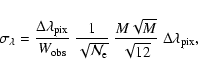
The error in the line center caused by counting statistics is given by
Bohlin et al. (1983, Eq. (A15)):
For Gaussian profiles, M can be equal to
2.5 FWHM
![]() ,
producing
,
producing
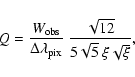
By analogy with the Connes procedure, we can characterize a line profile
by a dimensionless quality factor Q which is independent on the flux:
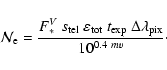
The total number of photoelectrons can be estimated from the specific
flux
![]() ergs s-1 cm-2 Hz-1
of a mv = 0 star outside the Earth's atmosphere
ergs s-1 cm-2 Hz-1
of a mv = 0 star outside the Earth's atmosphere![]() :
:
![]()
![]() 103 photon cm-2 s-1 Å-1.
Then
103 photon cm-2 s-1 Å-1.
Then
![]() is given by:
is given by:
Table 4:
Fundamental photon noise limits
![]() (in units of 10-5) for Fe II pairs of lines (
(in units of 10-5) for Fe II pairs of lines (
![]() )
from the
)
from the
![]() = 1.839 system toward Q 1101-264. The exposure time
= 1.839 system toward Q 1101-264. The exposure time
![]() and the total efficiency
and the total efficiency
![]() are set to 3600 s and 0.15, respectively.
are set to 3600 s and 0.15, respectively.
At 5500 Å, the UVES efficiency
![]() (Kaufer et al. 2004), and with a 3600 s exposure (
(Kaufer et al. 2004), and with a 3600 s exposure (
![]() ),
one expects a fundamental uncertainty of about 1-5 mÅ in
),
one expects a fundamental uncertainty of about 1-5 mÅ in
![]() for a mv = 16 QSO. Then, (11) provides, respectively, the fundamental noise of
for a mv = 16 QSO. Then, (11) provides, respectively, the fundamental noise of
![]()
![]() in
in
![]() for one measurement
of a Fe II pair of lines.
for one measurement
of a Fe II pair of lines.
The fundamental photon noise limits for Fe II pairs from the
![]() = 1.839 system are given in Table 4. The photon noise is computed with the
best-fitting parameters
N1 = 1.335
= 1.839 system are given in Table 4. The photon noise is computed with the
best-fitting parameters
N1 = 1.335 ![]() 1013 cm-2 and
b1 = 5.25 km s-1.
1013 cm-2 and
b1 = 5.25 km s-1.
Measurements from the present paper can be combined with the previous Fe II sample from
the
![]() = 1.15 system toward HE 0515-4414 (QRL) to increase statistics.
The normalized distribution (
= 1.15 system toward HE 0515-4414 (QRL) to increase statistics.
The normalized distribution (
![]()
![]() = 1) of the resulting 35
= 1) of the resulting 35
![]() values is plotted in Fig. 6 (histogram) along with two other recently published results of MFWDPW and CSPA which are shown by the dashed and dotted curves, respectively, assuming that the measured
values is plotted in Fig. 6 (histogram) along with two other recently published results of MFWDPW and CSPA which are shown by the dashed and dotted curves, respectively, assuming that the measured
![]() are normally distributed with the sample means and standard deviations
published in these papers. The vertical lines in this figure
mark the centers of the corresponding distributions.
The distribution shown by the histogram has the sample mean
are normally distributed with the sample means and standard deviations
published in these papers. The vertical lines in this figure
mark the centers of the corresponding distributions.
The distribution shown by the histogram has the sample mean
![]()
![]()
![]() =
=
![]() and the median
(
and the median
(
![]() )
)
![]() .
.
It is to be noted that at a given redshift the sample mean ![]()
![]()
![]() should
be the same within the uncertainty interval independently on the method or the sample used - provided the data are free from any systematics.
The results presented in Fig. 6 show, however, that
should
be the same within the uncertainty interval independently on the method or the sample used - provided the data are free from any systematics.
The results presented in Fig. 6 show, however, that
![]()
![]()
![]()
![]()
![]()
![]() .
The sample means of CSPA and our Fe II ensemble are in good agreement but
they differ from that of MFWDPW at the 95% significance level according to
the t-test
.
The sample means of CSPA and our Fe II ensemble are in good agreement but
they differ from that of MFWDPW at the 95% significance level according to
the t-test![]() . This discrepancy points to the systematic shift
which mimics the effect of varying
. This discrepancy points to the systematic shift
which mimics the effect of varying ![]() in the Keck/HIRES spectra.
To clarify the origin of this systematic shift, one needs more accurate measurements,
which can be carried out with higher spectral resolution and with more homogeneous samples.
in the Keck/HIRES spectra.
To clarify the origin of this systematic shift, one needs more accurate measurements,
which can be carried out with higher spectral resolution and with more homogeneous samples.
The comparison of the distribution widths in Fig. 6 reveals
that the standard deviation in the CSPA sample is exceptionally
small. For example, Fig. 1b in CSPA, where the
accuracy of wavelength calibration is checked through the relative velocity
shifts, ![]() ,
between the Fe II
,
between the Fe II
![]() and
and
![]() lines
lines![]() , shows the dispersion of
, shows the dispersion of
![]() km s-1. This uncertainty in wavelength calibration transforms into the error
km s-1. This uncertainty in wavelength calibration transforms into the error
![]() (see Eq. (12) in L04), i.e.,
in order to reach the error of the mean
(see Eq. (12) in L04), i.e.,
in order to reach the error of the mean
![]() (CSPA), one needs a sample of the size
(CSPA), one needs a sample of the size
![]() ,
which is not the case. Thus, the error of the mean
,
which is not the case. Thus, the error of the mean
![]() estimated by CSPA is in some disagreement with their Fig. 1b.
The scatter of
estimated by CSPA is in some disagreement with their Fig. 1b.
The scatter of
![]() in the Keck sample is about 2 times the
in the Keck sample is about 2 times the
![]() value of our combined Fe II sample.
value of our combined Fe II sample.
![\begin{figure}
\par\includegraphics[height=8.35cm,width=8cm,clip]{1827fig6.ps}\end{figure}](/articles/aa/full/2005/18/aa1827/img233.gif) |
Figure 6:
The distribution of
|
| Open with DEXTER | |
Future measurements of
![]() from astronomical observations
should be carried out with high precision to check the present Oklo result that
from astronomical observations
should be carried out with high precision to check the present Oklo result that ![]() was larger in the past,
was larger in the past,
![]()
![]() (Lamoreaux & Torgerson 2004). To reach the Oklo scale of
(Lamoreaux & Torgerson 2004). To reach the Oklo scale of ![]() -variation, one needs the accuracy of at least
-variation, one needs the accuracy of at least
![]() ,
which is 8 times higher than the accuracy set by the errors in the laboratory wavelengths (Sect. 4.1).
At first glance the Oklo level is unachievable in astronomical observations.
However, applying the SIDAM method to a few Fe II systems observed at different redshifts, one can omit the laboratory wavelengths from
,
which is 8 times higher than the accuracy set by the errors in the laboratory wavelengths (Sect. 4.1).
At first glance the Oklo level is unachievable in astronomical observations.
However, applying the SIDAM method to a few Fe II systems observed at different redshifts, one can omit the laboratory wavelengths from
![]() calculations. Such self-calibrating procedure, described by BSS, implies that the measured values of R(t), Eq. (7),
can be fitted to a linear function of cosmic time given in the form (cf. Eq. (6) in BSS):
calculations. Such self-calibrating procedure, described by BSS, implies that the measured values of R(t), Eq. (7),
can be fitted to a linear function of cosmic time given in the form (cf. Eq. (6) in BSS):
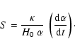
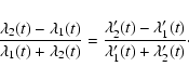
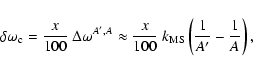
Equation (21) shows that for narrow lines (
![]() )
the error
)
the error
![]() decreases almost quadratically with
decreasing wavelength bin per pixel if
decreases almost quadratically with
decreasing wavelength bin per pixel if ![]() is fixed.
Therefore, if an efficient spectrograph with ten times the UVES dispersion and superior stability can be coupled to a 100 m class telescope, one would expect
is fixed.
Therefore, if an efficient spectrograph with ten times the UVES dispersion and superior stability can be coupled to a 100 m class telescope, one would expect
![]() 0.03-0.05 mÅ, and, thus, the precision of
0.03-0.05 mÅ, and, thus, the precision of ![]() 10-7 in the
10-7 in the
![]() measurements can be achieved. Then, with good statistics the Oklo result can be checked
at different redshifts.
measurements can be achieved. Then, with good statistics the Oklo result can be checked
at different redshifts.
If ![]() were indeed larger in the past, then the logarithmic derivative of
were indeed larger in the past, then the logarithmic derivative of ![]() in Eq. (24) is negative (since t decreases with increasing redshift) and we
would observe a positive slope S. Otherwise, if
in Eq. (24) is negative (since t decreases with increasing redshift) and we
would observe a positive slope S. Otherwise, if ![]() were smaller in the past,
S would be negative.
were smaller in the past,
S would be negative.
The main results of the present paper are as follows:
Acknowledgements
The authors are indebted to Ralf Quast for his valuable comments. S.A.L. gratefully acknowledges the hospitality of Osservatorio Astronomico di Trieste where this work was performed under the program COFIN 02 N 2002027319-001. The work of S.A.L. is supported by the RFBR grant No. 03-02-17522 and by the RLSS grant 1115.2003.2.


![\begin{displaymath}%
\tau^{(\ell)}_v = N_1~\sum^{n_{\rm s}}_{i=1}~r_{i,1}~{\cal V}\left[
(v - v_\ell - \Delta v_{i,1})/{b_i} \right],
\end{displaymath}](/articles/aa/full/2005/18/aa1827/img145.gif)
![\begin{displaymath}%
\chi^2(\theta) = \frac{1}{\nu}~\sum^{L}_{\ell=1}~\sum^{m_\e...
...ta) - {\cal F}^{\rm obs}_{\ell,j}
\right]^2/\sigma^2_{\ell,j},
\end{displaymath}](/articles/aa/full/2005/18/aa1827/img158.gif)