M. Khakian Ghomi - M. Bahmanabadi - J. Samimi
Department of Physics, Sharif university of Technology, PO Box 11365-9161, Tehran, Iran
Received 23 June 2004 / Accepted 3 November 2004
Abstract
Ultra-high-energy (E>100 TeV) Extensive Air Showers
(EASs) have been monitored for a period of five years (1997-2003), using a small array of scintillator detectors in Tehran,
Iran. The data have been analyzed taking into account the
dependence of source counts on zenith angle. During a calendar
year different sources come into the field of view of the detector
at varying zenith angles. Because of varying thickness of the
overlaying atmosphere, the shower count rate is extremely
dependent on zenith angle, which has been carefully analyzed over
time (2002, Exp. Astron., 13, 39). High energy gamma-ray sources from the
EGRET third catalogue where observed and the data were analyzed
using an excess method. Upper limits were obtained for a number of
EGRET sources, including 6 AGNs or probably AGNs and 4
unidentified sources.
Key words: instrumentation: detectors - methods: data analysis - catalogs - gamma rays: observations
Some other faint sources are in the mid-latitude region suggested to be associated with the Gould Belt (Gehrels et al. 2000), which underwent an intense star formation period about sixty million years ago (Grainer 2000; Harding & Zhang 2001). High latitude sources, of which there are about 50, might be galactic gamma-ray halo sources (Dixon et al. 1998) or unidentified sources that are thought to be extragalactic. These extragalactic EUI sources comprise Blasars and Active Galactic Nuclei (AGNs), galaxy clusters (Colafrancesco 2002), BL Lacerta objects (Torres et al. 2003) and other types.
Whether the EGRET sources emit at still higher energies, is an interesting question (Lamb & Macomb 1997). Gamma-rays with energies of about 100 TeV and more, entering the earth atmosphere, produce Extensive Air Showers (EASs) (Gaisser 1990) which could be observed by the detection of the secondary particles of the showers on the ground level (Bahmanabadi et al. 1998). Previous attempts have been reported from other EAS arrays (Amenomori et al. 2002, 2000; Borione et al. 1997; Alexandreas et al. 1993; McKay et al. 1993).
This paper
reports the results of a small particle detector array located at
the Sharif University of Technology in Tehran. This small array is a
prototype for a larger EAS array to be built at an altitude of 2600 m (![]() 756 g cm-2) at ALBORZ Observatory (AstrophysicaL
oBservatory for cOsmic Radiation on alborZ)
(http://sina.sharif.edu/~observatory/) near Tehran. The
prototype was installed on the roof of the physics department of
Sharif University of Technology in Tehran. In this work we present
the observational results for 10 EGRET third catalogue sources; we
describe the experimental setup in Sect. 2, the data analysis in
Sect. 3, the results in Sect. 4. Section 5 is devoted to a discussion
of the results.
756 g cm-2) at ALBORZ Observatory (AstrophysicaL
oBservatory for cOsmic Radiation on alborZ)
(http://sina.sharif.edu/~observatory/) near Tehran. The
prototype was installed on the roof of the physics department of
Sharif University of Technology in Tehran. In this work we present
the observational results for 10 EGRET third catalogue sources; we
describe the experimental setup in Sect. 2, the data analysis in
Sect. 3, the results in Sect. 4. Section 5 is devoted to a discussion
of the results.
![\begin{figure}
\par\includegraphics[width=12.5cm,clip]{1518fig1.eps}
\end{figure}](/articles/aa/full/2005/17/aa1518/img15.gif) |
Figure 1: Experimental set up and electronic circuits. |
| Open with DEXTER | |
When all of the scintillators have coincidence pulses, the TACs are trigged by the logic unit and the 3 time lags between the output signals of PMTs (4, 1), (2, 3) and (2, 1) are read out as parameters 1 to 3. So by this procedure an EAS event is logged.
Two different experimental configurations were used in the
experimental set up. The first (E1) and the second (E2)
experimental configurations were identical except for the size of
the array. In E1 the size is 8.75 m ![]() 8.75 m and in E2the size is 11.30 m
8.75 m and in E2the size is 11.30 m ![]() 11.30 m.
11.30 m.
The logged time lags between the scintillators and Greenwich Mean Time (GMT) of each EAS event were recorded as raw data. We synchronized our computer to GMT (http://www.timeanddate.com). Our electronic system has a recording capability of 18.2 times per second. If an EAS event occurs, its three time lags will be recorded and if it does not occur "zero'' will be recorded. Therefore the starting time of each experiment and the count of records gives us the GMT of each EAS event. Our detected EAS events are a mixture of cosmic-ray events and gamma-ray events. In E1 the total number of EAS events was 53 907 and the duration of the experiment was 501 460 s. So the mean event rate of the first experiment was 0.1075 events per second. The distribution of the time between successive events is in good agreement with an exponential function, indicating that the event sampling is completely random (Bahmanabadi et al. 2003). In E2 the total number of events was 173 765 and the duration of the second experiment was 2 902 857 s, so its mean event rate was 0.05986 events per seconds.
We refined the data to separate out acceptable events. Events are
acceptable if there is good coincidence between the four
scintillator pulses. We omitted the events with zenith angles more
than 60![]() .
Therefore after the separation we obtained
smaller data sets of 46 334 and 120 331 for E1 and E2respectively. Since we cannot determine the energy of the showers on
an event by event basis, we estimate our lower energy threshold by
comparing our event rate to a cosmic-ray integral spectrum
(Borione et al. 1997)
.
Therefore after the separation we obtained
smaller data sets of 46 334 and 120 331 for E1 and E2respectively. Since we cannot determine the energy of the showers on
an event by event basis, we estimate our lower energy threshold by
comparing our event rate to a cosmic-ray integral spectrum
(Borione et al. 1997)
| J(E) | = | ||
| (1) |
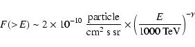 |
(2) |
The complete analysis procedure is as follows:
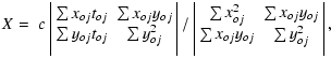
The local coordinates are zenith (z) and azimuth ![]() .
We
used the least-squares method (Mitsui et al. 1990) to calculate z and
.
We
used the least-squares method (Mitsui et al. 1990) to calculate z and ![]() .
It is assumed that the shower front could be
approximated
by a plane. So we obtain
.
It is assumed that the shower front could be
approximated
by a plane. So we obtain
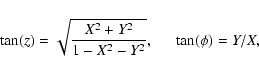 |
(3) |
 |
(4) | ||
 |
(5) |
A zenith angle cut off
![]() is implemented to increase the
significance.
is implemented to increase the
significance.
Figure 2a shows the azimuthal angle distribution of the EAS
events, which is nearly isotropic. A slight North-South anisotropy
is observed which is attributed to the geomagnetic field. We fitted
this distribution with a harmonic function as
follows: (Bahmanabadi et al. 2002)
 |
(6) |
Since the thickness of the atmosphere increases quickly with
increasing zenith angle z (Gaisser 1990), the number of EAS
events is strongly
related to z, as shown in Fig. 2b.
![\begin{figure}
\par\includegraphics[width=8.8cm,clip]{1518fig2.eps}
\end{figure}](/articles/aa/full/2005/17/aa1518/img36.gif) |
Figure 2:
Local coordinate distributions of, a) azimuth
" |
| Open with DEXTER | |
The equatorial coordinates (RA, Dec) are obtained from the local
coordinates (![]() ), GMT of each EAS event and geographical
latitude of the array. In this step the transformation relations
(http://aanda.u-strasbg.fr, Roy & Clarke), and the local
sidereal time of the starting point of the
experiment (http://tycho.usno.navy.mil/sidereal.html) were used.
), GMT of each EAS event and geographical
latitude of the array. In this step the transformation relations
(http://aanda.u-strasbg.fr, Roy & Clarke), and the local
sidereal time of the starting point of the
experiment (http://tycho.usno.navy.mil/sidereal.html) were used.
Then galactic coordinates (l, b) of each EAS event were derived
from the equatorial coordinates, for epoch 2000
(http://aanda.u-strasbg.fr). Figure 3 shows the distribution
of our data in galactic coordinates.
![\begin{figure}
\par\includegraphics[angle=-90,width=13cm,clip]{1518fig3.eps}
\end{figure}](/articles/aa/full/2005/17/aa1518/img42.gif) |
Figure 3:
EAS events map in 1
|
| Open with DEXTER | |
Table 1:
EGRET third catalogue sources observed by our array. ld and bd are displaced galactic coordinates,
![]() ,
,
![]() and
and
![]() are the statistical
significances
related to the first experiment, the second experiment and the sum
of the two,
are the statistical
significances
related to the first experiment, the second experiment and the sum
of the two, ![]() is the error angular radius,
is the error angular radius, ![]() is the
mean value of zenith angles of EASs for source and
"Flux'' is the number of EAS events for source. t1: AGN which has been
investigated before by CASA-MIA (Catanese et al. 1996), t2: sources with energy >1 GeV
(Lamb & Macomb 1997). Sources number 5 and 7 are "Mrk 421'' and "4C +10.45''
respectively.
is the
mean value of zenith angles of EASs for source and
"Flux'' is the number of EAS events for source. t1: AGN which has been
investigated before by CASA-MIA (Catanese et al. 1996), t2: sources with energy >1 GeV
(Lamb & Macomb 1997). Sources number 5 and 7 are "Mrk 421'' and "4C +10.45''
respectively.
For the coordinates calculation of each EAS event we have to know
estimated errors in these coordinates. These errors are due to
experimental error factors, which contain uncertainties in the
times and coordinates of each logged EAS event. The defined
distance between two scintillators was centre to centre and the
size of the scintillators was (
![]() cm3). The
accuracy of the coordinates of each scintillator is determined
within a few centimeters. So the error in the measurement of the
coordinates of secondary particles of each EAS event is
cm3). The
accuracy of the coordinates of each scintillator is determined
within a few centimeters. So the error in the measurement of the
coordinates of secondary particles of each EAS event is
![]() m.
m.
The errors in the time measurement of each EAS event
are due to the thickness of front plane of the secondary
particles, errors in the electronics and in GMT logging. The error
due to the first two factors was
![]() ns
(Bahmanabadi et al. 2002). The error in the logged time of each EAS event
was
ns
(Bahmanabadi et al. 2002). The error in the logged time of each EAS event
was
![]() s which is due to the recording rate and the
synchronizing of the computer. These errors cause uncertainties in
the coordinates of the investigated sources.
s which is due to the recording rate and the
synchronizing of the computer. These errors cause uncertainties in
the coordinates of the investigated sources.
The following quantities were calculated:
| (7) | |||
| (8) |
The errors in zenith and azimuth angles were obtained by
differentiating from Eqs. (7) and (8):
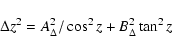 |
(9) |
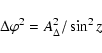 |
(10) |
If y is a generic
function of parameters u, v and T, then:
| y=y(u,v,T) | (11) |
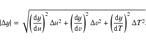 |
(12) |
The error in the observed solid angle of each source is
![]() and the equivalent error in the
angular radius is
and the equivalent error in the
angular radius is
![]() (
(
![]() )
)
The above analysis obtains as angular resolution for EAS event
individually. But there are many EAS events with different local
coordinates which contribute in the signature of each investigated
source. Therefore at first angular errors of all of the accumulated
EAS events in the galactic coordinates of the source were
calculated, then the mean value of these angular errors was chosen
as the angular error of the source. Since all of the accumulated EAS
events in the angular error region contribute to the source
signature, the previous calculations were repeated for all of the
accumulated EAS events in a circular region centered on the source
and with radius ![]() .
Finally the mean value of these EAS angular
errors is calculated as the angular error of each source in galactic
coordinates. Since the sides distances of the array are different in E1 and E2, the angular errors in these two experiments are
different. So for the calculation of the final result for each
source these angular errors were calculated separately for E1 and E2 and were weighted with the number of refined EAS events in the
related experiment. The final angular errors of the investigated
sources (
.
Finally the mean value of these EAS angular
errors is calculated as the angular error of each source in galactic
coordinates. Since the sides distances of the array are different in E1 and E2, the angular errors in these two experiments are
different. So for the calculation of the final result for each
source these angular errors were calculated separately for E1 and E2 and were weighted with the number of refined EAS events in the
related experiment. The final angular errors of the investigated
sources (![]() )
are shown in Table 1. Since these angular error
radii have a slight fluctuations around a mean value, we sampled
over l and b with a steps of 5 degrees from the FOV of the array and
calculated these radii to find the mean and standard deviation.
Therefore the mean and the standard deviation of the angular error
of the experiment were obtained from the angular errors of more than
1000 random points. With these steps we obtained
)
are shown in Table 1. Since these angular error
radii have a slight fluctuations around a mean value, we sampled
over l and b with a steps of 5 degrees from the FOV of the array and
calculated these radii to find the mean and standard deviation.
Therefore the mean and the standard deviation of the angular error
of the experiment were obtained from the angular errors of more than
1000 random points. With these steps we obtained
![]() as the mean angular error of
the experiment.
as the mean angular error of
the experiment.
![\begin{figure}
\par\includegraphics[angle=-90,width=13cm,clip]{1518fig4.eps}
\end{figure}](/articles/aa/full/2005/17/aa1518/img67.gif) |
Figure 4:
Exposure map of simulated events in 1
|
| Open with DEXTER | |
The energy range of the EAS events logged by the array is in the
range of 40 to 10 000 TeV. In this energy range the distribution of
cosmic rays is completely isotropic and homogeneous in the galaxy.
After correcting for the exposure effects, we looked for excess
emission that could be from gamma-ray sources. We used the third
EGRET catalogue (Hartman et al. 1999) as a reference. But some of EGRET
sources do not have acceptable events in the FOV of our array. We
counted the number of events, and the number of pixels and then
calculated the count per pixel related to each source. We note that
the mean count per pixel in the data map is 4.798. Of 151 EGRET
sources only 123 have counts per pixel of more than the
![]() ;
of these 98 have counts per pixel of more than 1.5 times the square root of the mean. So we started our investigations
with these 98 sources. A method of excess similar to the analysis
adopted by the Tibet EAS array, was adopted (Amenomori et al. 2002,
2000). In the first step we divided the data map
(Fig. 3) by the exposure map (Fig. 4) pixel by
pixel. In the obtained map, most non zero pixels are around 1 except
probable source pixels and pixels with higher fluctuations in the
data map, which are probably due to the small size of the data set.
To eliminate the fluctuating pixels we multiplied the new map by 4.798 to obtained a raw exposure-corrected map. In this step we
added counts of all pixels of the raw corrected map. The number must
be very near to 166 665 so with this restriction we obtained a lower
limit 0.0750 for eliminating pixels with lower count in the exposure
map, and the final
exposure corrected map was obtained; it is shown in Fig. 5.
;
of these 98 have counts per pixel of more than 1.5 times the square root of the mean. So we started our investigations
with these 98 sources. A method of excess similar to the analysis
adopted by the Tibet EAS array, was adopted (Amenomori et al. 2002,
2000). In the first step we divided the data map
(Fig. 3) by the exposure map (Fig. 4) pixel by
pixel. In the obtained map, most non zero pixels are around 1 except
probable source pixels and pixels with higher fluctuations in the
data map, which are probably due to the small size of the data set.
To eliminate the fluctuating pixels we multiplied the new map by 4.798 to obtained a raw exposure-corrected map. In this step we
added counts of all pixels of the raw corrected map. The number must
be very near to 166 665 so with this restriction we obtained a lower
limit 0.0750 for eliminating pixels with lower count in the exposure
map, and the final
exposure corrected map was obtained; it is shown in Fig. 5.
![\begin{figure}
\par\includegraphics[angle=-90,width=13cm,clip]{1518fig5.eps}
\end{figure}](/articles/aa/full/2005/17/aa1518/img70.gif) |
Figure 5: Corrected exposure map extracted by pixel-by-pixel division of the data map (Fig. 3) by the exposure map (Fig. 4). |
| Open with DEXTER | |
The obtained map was fairly uniform in the FOV of our array in
galactic coordinates. Next we investigated the remaining faint
inhomogeneity in the corrected map that could be conditionally
attributed to the existence of gamma-ray sources. To estimate the
significance of an individual source we added all corrected EAS
events,
![]() ,
within a radius
,
within a radius
![]() from the source
position. The number of pixels,
from the source
position. The number of pixels, ![]() ,
within this region was also
counted. The total number of background counts,
,
within this region was also
counted. The total number of background counts,
![]() ,
was found
from the pixels that fall within an outer radius of 2
,
was found
from the pixels that fall within an outer radius of 2![]() and an
inner radius
and an
inner radius
![]() from the source position. The number of
background pixels,
from the source position. The number of
background pixels, ![]() ,
was also counted too. The statistical
significance of the source was obtained using the Li & Ma method
(Li & Ma 1983).
,
was also counted too. The statistical
significance of the source was obtained using the Li & Ma method
(Li & Ma 1983).
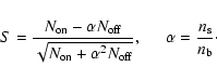 |
(13) |
 |
(14) |
![\begin{figure}
\par\includegraphics[width=8.8cm,clip]{1518fig6.eps}
\end{figure}](/articles/aa/full/2005/17/aa1518/img78.gif) |
Figure 6:
Distribution of frequency of a) 98 000 virtual random sources and
b) 98 EGRET
sources in the FOV of our array in galactic coordinates versus their statistical
significance.
|
| Open with DEXTER | |
 |
(15) |
Our exposure-corrected map has not bright source signatures, so we
used the third EGRET catalogue as a reference for searching some
sources in our energy range. But the EGRET energy range is from 100 MeV to 30 GeV and our energy range is from 40 TeV to 10 000 TeV. So
to be detectable in our data these sources should have a spectrum
that spreads from at least the EGRET energy range to our energy
range, such as blazars, BL Lac objects, Flat-spectrum radio quasars
or etc. Since these sources do not usually have exactly the same
position in different energy ranges, we searched a position one
degree away from these sources. This displaced l and b are shown in
Table 1 for each source. It means that around each source with a
statistical significance of more than 1 we tried 8 (
![]() ) pixels and chose the location with the highest statistical
significance.
) pixels and chose the location with the highest statistical
significance.
The rotation axis of the Earth passes near the star Polaris; the
angular difference between Polaris and the rotation axis is
approximately 5 times smaller than our mean angular accuracy (
![]() )
in galactic coordinates. So in this analysis Polaris
is considered to be on the rotation axis of the Earth. The
longitude and latitude of Polaris in galactic coordinates are
)
in galactic coordinates. So in this analysis Polaris
is considered to be on the rotation axis of the Earth. The
longitude and latitude of Polaris in galactic coordinates are
![]() ,
17' and
,
17' and
![]() ,
28' respectively. The
geographical latitude of Tehran is about
,
28' respectively. The
geographical latitude of Tehran is about
![]() N, so the
angle between the zenith of the array and Polaris in Tehran is
about
N, so the
angle between the zenith of the array and Polaris in Tehran is
about
![]() .
We selected events with zenith angles less
than
.
We selected events with zenith angles less
than
![]() for the analysis which is deduced from
Fig. 2b and therefore, Polaris and regions around it
are observable only with High zenith EAS events. From
Fig. 2b it can be seen that the best observable region
is for zenith angle between
for the analysis which is deduced from
Fig. 2b and therefore, Polaris and regions around it
are observable only with High zenith EAS events. From
Fig. 2b it can be seen that the best observable region
is for zenith angle between
![]() to
to
![]() of zenith
angles. In Fig. 3 we show that Galactic longitudes smaller
than
of zenith
angles. In Fig. 3 we show that Galactic longitudes smaller
than
![]() and larger than
and larger than
![]() are less well observable. In other
words, given the location of the array there are two different
observable regions in galactic coordinates. Galactic latitudes
smaller than
are less well observable. In other
words, given the location of the array there are two different
observable regions in galactic coordinates. Galactic latitudes
smaller than
![]() and larger than
and larger than
![]() are
also less suitable to observe regions too.
are
also less suitable to observe regions too.
With the procedure mentioned in Sect. 3.7. we searched for sources with statistical significance >1.5, and we found thirteen sources of which five of them have a significance >2. To avoid possible fluctuations we repeated our search. We searched these displaced sources in E1 and E2 separately. But at this stage, because of the small size of these data sets, specially in E1 we selected sources with a significance >1. Ten sources remained which have a statistical significance >1 in E1 and E2and >1.5 in the sum; these are listed in Table 1. Fortunately five of these sources are AGNs, one is a probable AGN and four are unidentified sources. Note that out of 271 sources of the third EGRET catalogue only 66 are AGNs.
It seems that the radial distribution of the number of counts per
pixel for each source naturally must be close to a gaussian
distribution over a flat back ground. We selected eight regions with
approximately the same number of pixels for each source. The first
region is a circle with radius
![]() .
The second region is
a ring with inner radius
.
The second region is
a ring with inner radius
![]() and outer radius
and outer radius
![]() and so on. The distribution of the mean counts per
pixel around 98 000 virtual random sources and 10 most significant
EGRET sources is shown in Fig. 7. These distributions
fitted a gaussian function over a flat distribution as follows:
and so on. The distribution of the mean counts per
pixel around 98 000 virtual random sources and 10 most significant
EGRET sources is shown in Fig. 7. These distributions
fitted a gaussian function over a flat distribution as follows:
 |
(16) |
![\begin{figure}
\par\includegraphics[width=8.8cm,clip]{1518fig7.eps}
\end{figure}](/articles/aa/full/2005/17/aa1518/img94.gif) |
Figure 7: Distribution of mean count per pixel of a) 98 000 virtual random sources and b) 10 EGRET sources of Table 1 versus error radial distance from the centre of the related sources. |
| Open with DEXTER | |
![\begin{figure}
\par\includegraphics[angle=-90,width=12cm,clip]{1518fig8.eps}
\end{figure}](/articles/aa/full/2005/17/aa1518/img95.gif) |
Figure 8: Map of EGRET sources with statistical significance more than 1.5 in galactic coordinates. The numbered sources are listed in Table 1. |
| Open with DEXTER | |
There has been considerable effort worldwide to detect gamma-ray
sources via the EAS technique. From a variety of arguments we
suspect that some of the EGRET sources would be detectable at very
high energies. In this work, we are limited to a discussion of a few
sources with relatively small statistical significance. Our values
for the statistical significance do not constitute a confident
detection limit, our main object was to get an indication of the
possibility of detecting some unidentified EGRET sources in the
high-TeV range. Of these sources listed in Table 1, we suspect that
nine may be extra galactic (
![]() )
(Gehrels et al. 2000) and
only one is in the galactic region (
)
(Gehrels et al. 2000) and
only one is in the galactic region (
![]() )
and this
one is an AGN in the third EGRET catalogue list too. Four of our ten
sources were investigated before with CASA-MIA (Catanese et al. 1996) and
two of them were GEV EGRET sources (Lamb & Macomb 1997). Therefore we might
expect that as many as four of these unidentified sources could
indeed be emitters at high energy and might be AGNs.
)
and this
one is an AGN in the third EGRET catalogue list too. Four of our ten
sources were investigated before with CASA-MIA (Catanese et al. 1996) and
two of them were GEV EGRET sources (Lamb & Macomb 1997). Therefore we might
expect that as many as four of these unidentified sources could
indeed be emitters at high energy and might be AGNs.
Some of our observed sources overlap one another (Fig. 8), so a complete and accurate analysis procedure should incorporate the maximum likelihood method (Mattox et al. 1996). We must also emphasize that our experiment cannot distinguish between gamma-ray and cosmic-ray initiated air showers, and so we used the excess method to carry out a search for very high energy gamma-ray emission. After the analysis we understood that the recording rate of our computer is very important and we have to increase it to reduce the angular error radius of observable sources. In our future site at 2600 m above sea level (http://sina.sharif.edu/~observatory), we are constructing underground tunnels which will provide us with ample space to deploy muon detectors. The detection of muons in air showers should be a powerful way to discriminate between cosmic-ray and gamma-ray air showers.
Acknowledgements
This research was supported by a grant from the national research council of Iran for basic sciences. The authors wish to thank Dr. Dipen Bhattacharya at University of California, Riverside and Prof. Rene A. Ong at University of California, Los Angeles for their many constructive comments. The authors wish to thank the anonymous referee for his/her many constructive comments too.