A&A 429, 807-818 (2005)
DOI: 10.1051/0004-6361:20041168
Cosmological parameters from supernova observations: A critical comparison
of three data sets
T. R. Choudhury 1 -
T. Padmanabhan 2
1 - SISSA/ISAS, via Beirut 2-4, 34014 Trieste, Italy
2 -
IUCAA, Ganeshkhind, Pune, 411 007, India
Received 27 April 2004 / Accepted 15 September 2004
Abstract
We extend our previous analysis of cosmological supernova type Ia data
(Padmanabhan & Choudhury 2003) to include three recent compilation of data sets.
Our analysis ignores the possible correlations and systematic effects
present in the data and concentrates mostly on some key theoretical
issues.
Among the three data sets, the first set
consists of 194 points obtained from various
observations while the second
discards some of the points from the
first one because of large uncertainties
and
thus consists of 142 points. The third data set is obtained
from the second by adding the latest 14 points observed through HST.
A careful comparison of these different data sets help us to draw
the following conclusions: (i) All the three data sets strongly rule out
non-accelerating models.
Interestingly, the first and the second data sets favour a closed
universe; if
 ,
then the
probability of obtaining models with
,
then the
probability of obtaining models with
 is
is
 0.97.
Hence these data sets are in
mild disagreement with the "concordance'' flat model. However, this
disagreement is reduced (the probability of obtaining models with
being
0.97.
Hence these data sets are in
mild disagreement with the "concordance'' flat model. However, this
disagreement is reduced (the probability of obtaining models with
being  0.9) for the third data set, which
includes the most recent points observed by HST around
1 < z < 1.6.
(ii) When the first data set is divided into two separate
subsets consisting of low (z < 0.34) and high (z > 0.34)
redshift supernova, it
turns out that these two subsets, individually, admit
non-accelerating models with
zero dark energy because of different magnitude zero-point values
for the different subsets.
This can also be seen when the data is analysed while allowing
for possibly different
magnitude zero-points for the two redshift subsets.
However, the non-accelerating models
seem to be ruled out using only the low redshift data for
the other two data sets, which have
less uncertainties.
(iii) We have also
found that it is quite difficult to measure the
evolution of the dark energy equation of state wX(z) though
its present value can be constrained quite well.
The best-fit value seems to mildly favour a dark energy component
with current equation of state wX < -1, thus opening
the possibility of existence of more exotic forms of matter. However,
the data is still consistent with the
the standard cosmological constant at 99 per cent confidence level
for
0.9) for the third data set, which
includes the most recent points observed by HST around
1 < z < 1.6.
(ii) When the first data set is divided into two separate
subsets consisting of low (z < 0.34) and high (z > 0.34)
redshift supernova, it
turns out that these two subsets, individually, admit
non-accelerating models with
zero dark energy because of different magnitude zero-point values
for the different subsets.
This can also be seen when the data is analysed while allowing
for possibly different
magnitude zero-points for the two redshift subsets.
However, the non-accelerating models
seem to be ruled out using only the low redshift data for
the other two data sets, which have
less uncertainties.
(iii) We have also
found that it is quite difficult to measure the
evolution of the dark energy equation of state wX(z) though
its present value can be constrained quite well.
The best-fit value seems to mildly favour a dark energy component
with current equation of state wX < -1, thus opening
the possibility of existence of more exotic forms of matter. However,
the data is still consistent with the
the standard cosmological constant at 99 per cent confidence level
for
 .
.
Key words: supernovae: general - cosmology: miscellaneous -
cosmological parameters
Current cosmological observations, particularly those
of supernova type Ia, show a strong signature of
the existence of a
dark energy component with negative pressure
(Perlmutter et al. 1999; Riess 2000; Riess et al. 1998). The most obvious
candidate for this dark energy is the cosmological constant (with
the equation of state
 ), which, however,
raises several theoretical difficulties (for reviews,
see Sahni & Starobinsky 2000; Peebles & Ratra 2003; Padmanabhan 2003).
This has led to
models for dark energy component
which evolves with time (Barreiro et al. 2000; Zlatev et al. 1999; Brax & Martin 1999; Wetterich 1988; Frieman et al. 1995; Ferreira & Joyce 1998; Ratra & Peebles 1988; Bilic et al. 2002; Brax & Martin 2000; Albrecht & Skordis 2000; Urena-Lopez & Matos 2000).
), which, however,
raises several theoretical difficulties (for reviews,
see Sahni & Starobinsky 2000; Peebles & Ratra 2003; Padmanabhan 2003).
This has led to
models for dark energy component
which evolves with time (Barreiro et al. 2000; Zlatev et al. 1999; Brax & Martin 1999; Wetterich 1988; Frieman et al. 1995; Ferreira & Joyce 1998; Ratra & Peebles 1988; Bilic et al. 2002; Brax & Martin 2000; Albrecht & Skordis 2000; Urena-Lopez & Matos 2000).
Currently, there is a tremendous amount of activity
going on in trying to determine the equation of state wX(z) and
other cosmological parameters from
observations of high redshift type Ia supernova
(Weller & Albrecht 2002; Podariu et al. 2001; McInnes 2004; Alcaniz 2004; Rowan-Robinson 2002; Wang & Lovelace 2001; Saini et al. 2000; Bertolami 2004; Wang & Tegmark 2004; Dev et al. 2004; Gong et al. 2004; Caresia et al. 2004; Novello et al. 2003; Gong 2004; Padmanabhan & Choudhury 2003; Weller & Albrecht 2001; Minty et al. 2002; Goliath et al. 2001; Astier 2000; Knop et al. 2003; Maor et al. 2002; Chae et al. 2004; Gerke & Efstathiou 2002; Corasaniti & Copeland 2002; Wang & Mukherjee 2004; Linder & Jenkins 2003; Wang & Garnavich 2001; Visser 2004; Gong & Duan 2004; Trentham 2001; Leibundgut 2001; Kujat et al. 2002; Garnavich et al. 1998; Zhu & Fujimoto 2003; Gong & Chen 2004; Alam et al. 2004; Szydlowski & Czaja 2004; Lima & Alcaniz 2004; Bertolami et al. 2004; Zhu et al. 2004; Alcaniz & Pires 2004; Nesseris & Perivolaropoulos 2004).
While there has been a considerable activity in this field,
one should keep in mind that there are several theoretical
degeneracies in the Friedmann model, which can
limit the determination of wX(z). To understand
this, note that the only
non-trivial metric function in a Friedmann universe is the
Hubble parameter H(z) (besides the curvature of the spatial
part of the metric), which is related
to the total
energy density in the universe.
Hence, it is not possible to determine the energy
densities of individual components of energy densities in the
universe from any geometrical observation. For example,
if we assume a flat universe,
and further assume that
the only energy densities present are those corresponding to
the non-relativistic dust-like
matter and dark energy, then we need to know
 of
the dust-like matter and H(z) to a very high accuracy in order
to get a handle on
of
the dust-like matter and H(z) to a very high accuracy in order
to get a handle on  or wX of the dark energy. This can be
a fairly strong degeneracy for determining wX(z) from observations.
or wX of the dark energy. This can be
a fairly strong degeneracy for determining wX(z) from observations.
Recently, we discussed
certain questions related to the
determination of the nature of
dark energy component from observations of high redshift supernova
in Padmanabhan & Choudhury (2003, hereafter Paper I).
In the above work, we
reanalyzed the supernova data using very simple
statistical tools in order to focus attention on
some key issues. The analysis of the data were
intentionally kept simple as
we subscribe to the point of
view that any result which cannot be revealed by a simple
analysis of data, but arises
through a more complex statistical procedure, is inherently
suspect and a conclusion as
important as the existence of dark energy with
negative pressure should pass such a test. The key results
of our previous analysis were:
 Even if the precise
value of
or the equation of state wX(z) is known from
observations, it is not possible to determine the nature
(or, say, the Lagrangian) of
the unknown dark energy source using only kinematical
and geometrical measurements.
For example,
if one assumes that the dark energy arises from a scalar field, then
it is possible to come up with
scalar field Lagrangians of different forms leading to same wX(z).
As an explicit example, we considered
two Lagrangians, one corresponding to quintessence
(Peebles & Ratra 1988; Zlatev et al. 1999; Ratra & Peebles 1988) and
the other corresponding to the tachyonic scalar fields
(Mukohyama 2002; Shiu & Wasserman 2002; Padmanabhan 2002; Padmanabhan & Choudhury 2002; Bagla et al. 2003; Fairbairn & Tytgat 2002; Frolov et al. 2002; Feinstein 2002; Gibbons 2002).
These two fields are quite different in terms of their intrinsic
properties; however,
it is possible to make both the Lagrangians
produce a given wX(a) by choosing the potential functions in
the corresponding Lagrangians (for explicit examples and forms
of potential functions,
see Padmanabhan (2002); Paper I).
Even if the precise
value of
or the equation of state wX(z) is known from
observations, it is not possible to determine the nature
(or, say, the Lagrangian) of
the unknown dark energy source using only kinematical
and geometrical measurements.
For example,
if one assumes that the dark energy arises from a scalar field, then
it is possible to come up with
scalar field Lagrangians of different forms leading to same wX(z).
As an explicit example, we considered
two Lagrangians, one corresponding to quintessence
(Peebles & Ratra 1988; Zlatev et al. 1999; Ratra & Peebles 1988) and
the other corresponding to the tachyonic scalar fields
(Mukohyama 2002; Shiu & Wasserman 2002; Padmanabhan 2002; Padmanabhan & Choudhury 2002; Bagla et al. 2003; Fairbairn & Tytgat 2002; Frolov et al. 2002; Feinstein 2002; Gibbons 2002).
These two fields are quite different in terms of their intrinsic
properties; however,
it is possible to make both the Lagrangians
produce a given wX(a) by choosing the potential functions in
the corresponding Lagrangians (for explicit examples and forms
of potential functions,
see Padmanabhan (2002); Paper I).
Although
the full data set of supernova observations
strongly rule out models without dark energy,
the high and low redshift
data sets, individually, admit non-accelerating models with
zero dark energy. It is not surprising that the high redshift data
is consistent with non-accelerating models as the universe is in its
decelerating phase at those redshifts.
On the other hand, though the acceleration
of the universe is a low redshift phenomenon, the non-accelerating
models could not be ruled out using low redshift data alone because of
large errors.
Given the small data set, any possible evolution
in the absolute magnitude of the supernovae, if detected,
might have allowed the data to be consistent with the non-accelerating models.
We introduced two parameters, which
can be obtained entirely from theory,
to study the sensitivity of the luminosity distance on wX.
Using these two parameters, we argued that although
one can determine the present value of wX accurately from
the data, one cannot constrain the evolution of wX. The situation
is worse if we add the uncertainties in determining
.
All the above conclusions were obtained by analysing only 55
supernova data points from a very simple point of view.
In recent times, data points from various sets of observations have been
compiled taking into account the calibration errors and other uncertainties.
This enables us to repeat our analysis for much larger data sets, and
see how robust are the conclusions of Paper I with respect to
the choice of the data points. In this paper, we will compare
three such data sets, which differ in their selection criteria
for data points and redshift range covered.
The structure of the paper is as follows: in the next section, we
describe the three data sets used in this paper,
and then analyse them for models
with non-relativistic dust-like matter and
cosmological constant. Some key points
regarding the importance of low and high redshift data are discussed.
In Sect. 3, we briefly discuss the constraints on the
dark energy equation of state and its evolution. The results are
summarized in Sect. 4. Finally, the effect of our
extinction-based selection criterion on the determination of cosmological
parameters is discussed in the appendix.
2 Recent supernova data and their analysis
We begin with a brief outline of the method of our analysis
of the supernova data.
The observations essentially
measure the apparent magnitude m of a supernova at peak brightness
which, after correcting for galactic extinction and possible
K-correction, is related to the
luminosity distance  of the supernova through
 |
(1) |
where
 |
(2) |
and
 |
(3) |
The parameter M is the absolute magnitude of the supernovae after correcting
for supernova light curve width - luminosity
correlation (Perlmutter et al. 1997; Phillips et al. 1999; Riess et al. 1996).
After applying the above correction, M, and hence  ,
is
believed to be constant
for all supernovae of type Ia.
,
is
believed to be constant
for all supernovae of type Ia.
For our analysis, we
consider three sets of data available in the literature at present.
For completeness, we describe the data sets in detail:
(i) TONRY: in this data set we start with the 230 data points listed in
Tonry et al. (2003) alongwith the 23 points
from Barris et al. (2004).
These data points are compiled and calibrated from a wide range of different
observations.
For obtaining the best-fit cosmological model from the data, one
should keep in mind that the very low-redshift points might be affected
by peculiar motions, thus making the measurement of
the cosmological redshift uncertain; hence we consider only those
points which have z > 0.01. Further, since one is not sure about
the host galaxy extinction  ,
we do not consider
points which have
,
we do not consider
points which have
 .
The effect of this selection criterion based on the extinction, is discussed
in the appendix.
Thus
for our final
analysis, we are left with only 194 points
(identical to what is used in Barris et al. 2004), which
is more than thrice compared to what was used in Paper I.
.
The effect of this selection criterion based on the extinction, is discussed
in the appendix.
Thus
for our final
analysis, we are left with only 194 points
(identical to what is used in Barris et al. 2004), which
is more than thrice compared to what was used in Paper I.
The supernova data points in Tonry et al. (2003) and Barris et al. (2004)
are listed in terms of the luminosity distance
 |
(4) |
alongwith
the corresponding errors
 .
Note
that the quantity
.
Note
that the quantity  is obtained from observations
by assuming some value of .
This assumed value
of
(denoted by
is obtained from observations
by assuming some value of .
This assumed value
of
(denoted by
 in Eq. (4))
does not necessarily represent the "true'' ,
and hence
one has to keep it as a free parameter while fitting the data.
in Eq. (4))
does not necessarily represent the "true'' ,
and hence
one has to keep it as a free parameter while fitting the data.
Any model of cosmology will predict the
theoretical value
 with some undetermined parameters
 (which may be, for example,
 ). The best-fit model
is obtained by minimizing the quantity
). The best-fit model
is obtained by minimizing the quantity
![\begin{displaymath}\chi_1^2 = \sum_{i=1}^M \left[
\frac{\mu_1(z_i)
- {\cal M}_1...
...10}Q_{\rm th}(z_i; c_{\alpha})}{\sigma_{\mu_1}(z_i)}
\right]^2
\end{displaymath}](/articles/aa/full/2005/03/aa1168/img37.gif) |
(5) |
where
 |
(6) |
is a free parameter representing the difference between the
actual
and its assumed value
in the data. To take into account the uncertainties arising because of
peculiar motions at low redshifts, we add an
uncertainty of
 km s-1 to the distance error
(Tonry et al. 2003), i.e.,
km s-1 to the distance error
(Tonry et al. 2003), i.e.,
 |
(7) |
Note that this correction is most effective at low redshifts (i.e.,
for small values of  ). The minimization of (5) is done with respect to the parameter
 and the cosmological parameters
.
and the cosmological parameters
.
(ii) RIESS(w/o HST): recently, Riess et al. (2004)
have compiled a set of supernova data
points from various sources
with reduced calibration errors arising from systematics. In
particular, they have discarded various points
from the TONRY data set where the classification of the supernova
was not certain or the
photometry was incomplete - it is claimed that
this has increased
the reliability of the sample. The most reliable set of data,
named as "gold'', contain
142 points from previously published data, plus 14 points
discovered recently using HST (Riess et al. 2004).
Our second data set consists of 142 points from the above "gold'' sample of
(Riess et al. 2004), which does not include
the latest HST data (hence the name RIESS(w/o HST)).
Essentially, this
data set is similar to the TONRY data set in terms of the covered
redshift range, but is supposed to be more "reliable'' in terms
of calibration and other uncertainties.
We would like to mention here that the data points in (Riess et al. 2004) are
given in terms of the distance modulus
 |
(8) |
which differs from the previously defined quantity
in Eq. (4)
by a constant factor. Consequently, the  is
calculated from
is
calculated from
![\begin{displaymath}\chi_2^2 = \sum_{i=1}^M \left[
\frac{\mu_2(z_i)
- {\cal M}_2...
...10}Q_{\rm th}(z_i; c_{\alpha})}{\sigma_{\mu_2}(z_i)}
\right]^2
\end{displaymath}](/articles/aa/full/2005/03/aa1168/img44.gif) |
(9) |
where
 |
(10) |
Note that the errors
 quoted in Riess et al. (2004)
already take into account the effects of peculiar motions.
quoted in Riess et al. (2004)
already take into account the effects of peculiar motions.
(iii) RIESS: our third data set consists of all the 156 points in the
"gold'' sample of (Riess et al. 2004), which includes the latest points
observed by HST. The main difference of this set from the previous two is that
this covers the previously
unpopulated redshift range
1 < z < 1.6.
Before starting our analysis, we would like to caution the reader about
two very important points. First, the errors
 used above do
not contain uncertainties because of systematics. Any rigorous
statistical analysis of the supernova data for determining the
cosmological parameters must take into account the systematic errors.
The errors might arise because of calibration uncertainties,
K-correction, Malmquist bias,
gravitational lensing or the evolutionary effects
(Goobar et al. 2002a,b; Linder & Huterer 2003; Wang 2004; Linder 2004; Kim et al. 2004; Caresia et al. 2004; Perlmutter & Schmidt 2003; Huterer et al. 2004).
Including
such errors into the analysis requires much involved analysis. Once
these systematic errors are included, the errors on the cosmological
parameter estimations might be higher than what will be reported
in this paper. In this respect,
we would also like to add that the data sets RIESS and
RIESS(w/o HST) are supposed
to reduce some of the systematic and calibration uncertainties in data.
used above do
not contain uncertainties because of systematics. Any rigorous
statistical analysis of the supernova data for determining the
cosmological parameters must take into account the systematic errors.
The errors might arise because of calibration uncertainties,
K-correction, Malmquist bias,
gravitational lensing or the evolutionary effects
(Goobar et al. 2002a,b; Linder & Huterer 2003; Wang 2004; Linder 2004; Kim et al. 2004; Caresia et al. 2004; Perlmutter & Schmidt 2003; Huterer et al. 2004).
Including
such errors into the analysis requires much involved analysis. Once
these systematic errors are included, the errors on the cosmological
parameter estimations might be higher than what will be reported
in this paper. In this respect,
we would also like to add that the data sets RIESS and
RIESS(w/o HST) are supposed
to reduce some of the systematic and calibration uncertainties in data.
Second, our simple frequentist analysis
holds good only when the errors
are Gaussian and
uncorrelated. While considerable amount of analysis
exist in the literature working with these approximations,
there are various systematics because of which such approximations
do not hold true.
For example, the uncertainties in calibrating the data would surely
introduce correlations in the errors (Kim et al. 2004). Similarly, uncertainties
in the host galaxy extinction would introduce non-Gaussian asymmetric
errors. Neglecting such effects might result in lower errors on the
estimated values of the cosmological parameters.
Note that the main thrust of our analysis is to study some of the theoretical
degeneracies inherent in any geometrical observations, in particular the
supernova data, which are not adequately stressed elsewhere.
Of course, this study can be complemented by other analyses
which actually deal with quality and reliability of data,
validity of error estimates, hidden correlations,
nature of statistical analysis etc.
All of these are important, but in order to make some key points
we have attempted to restrict the domain of our exploration.
Keeping this in mind, we believe that the simple
(non-rigorous)
analysis should be adequate.
![\begin{figure}
\par\includegraphics[angle=270,width=8cm,clip]{1168fig1.ps}
\end{figure}](/articles/aa/full/2005/03/aa1168/Timg48.gif) |
Figure 1:
Comparison between various flat models and
the observational data.
The observational data points, shown with error-bars, are obtained
from the "gold'' sample of Riess et al. (2004). The most recent
points, obtained from HST, are shown in red. (This figure is available in color in electronic form.) |
| Open with DEXTER |
![\begin{figure}
\par\includegraphics[angle=270,width=17cm,clip]{1168fig2.ps}
\end{figure}](/articles/aa/full/2005/03/aa1168/Timg50.gif) |
Figure 2:
The observed supernova data points in the
 plane for
flat models. The error bars for the data points
are correlated (see text for detailed description). The solid
curves, from bottom to top,
are for flat cosmological models with
plane for
flat models. The error bars for the data points
are correlated (see text for detailed description). The solid
curves, from bottom to top,
are for flat cosmological models with
 respectively.
The left, middle and right panels show data points for the data sets RIESS, RIESS(w/o HST) and TONRY respectively. The vertical dashed line
shows the redshift z = 0.34.
respectively.
The left, middle and right panels show data points for the data sets RIESS, RIESS(w/o HST) and TONRY respectively. The vertical dashed line
shows the redshift z = 0.34. |
| Open with DEXTER |
![\begin{figure}
\par\includegraphics[angle=270,width=15cm,clip]{1168fig3.ps}
\end{figure}](/articles/aa/full/2005/03/aa1168/Timg51.gif) |
Figure 3:
Confidence region
ellipses in the
 plane for flat models with
non-relativistic matter and a cosmological constant. The
ellipses corresponding to the 68, 90 and 99 per cent confidence regions are shown.
The top, middle and bottom rows show data points for the data sets RIESS, RIESS(w/o HST) and TONRY respectively.
In the left panels, all the data points in the data set are used.
In the middle panel, data
points with z < 0.34 are used, while in the right panel, we have used
data points with z > 0.34. We have indicated the best-fit values of
and plane for flat models with
non-relativistic matter and a cosmological constant. The
ellipses corresponding to the 68, 90 and 99 per cent confidence regions are shown.
The top, middle and bottom rows show data points for the data sets RIESS, RIESS(w/o HST) and TONRY respectively.
In the left panels, all the data points in the data set are used.
In the middle panel, data
points with z < 0.34 are used, while in the right panel, we have used
data points with z > 0.34. We have indicated the best-fit values of
and
 (with 1
 errors).
 |
| Open with DEXTER |
Let us start our analysis with the flat models where
 ,
which are currently favoured strongly
by CMBR data (for recent WMAP results, see Spergel et al. 2003).
Our simple analysis for the most recent RIESS data set, with two free
parameters (
,
which are currently favoured strongly
by CMBR data (for recent WMAP results, see Spergel et al. 2003).
Our simple analysis for the most recent RIESS data set, with two free
parameters (
 ), gives
a best-fit value of
(after marginalizing
over
), gives
a best-fit value of
(after marginalizing
over
 )
to be
)
to be
 (all the errors quoted in this paper are 1).
This matches with the value
(all the errors quoted in this paper are 1).
This matches with the value
 obtained by Riess et al. (2004).
In comparison, the best-fit
for flat models
was found to be
obtained by Riess et al. (2004).
In comparison, the best-fit
for flat models
was found to be
 in Paper I - thus there is
a clear improvement in the errors because of increase in the
number of data points although the best-fit value does not change.
The comparison between three flat models and
the observational data from the RIESS data set
is shown in in Fig. 1.
in Paper I - thus there is
a clear improvement in the errors because of increase in the
number of data points although the best-fit value does not change.
The comparison between three flat models and
the observational data from the RIESS data set
is shown in in Fig. 1.
To see the accelerating phase of the universe more clearly,
let us display
the data as the phase portrait of the universe in the
 plane.
Though the procedure for
doing this is described in Paper I
(see also Daly & Djorgovski 2003), we
would like to discuss some aspects of the procedure in
detail to emphasize a different approach we have used
here in estimating the errors.
plane.
Though the procedure for
doing this is described in Paper I
(see also Daly & Djorgovski 2003), we
would like to discuss some aspects of the procedure in
detail to emphasize a different approach we have used
here in estimating the errors.
Each of the three sets of observational data used in this paper can be fitted
by the function of simple form
![\begin{displaymath}m_{\rm fit}(z)
= a_1 + 5 \log_{10} \left[\frac{z (1 + a_2 z)}{1 + a_3 z}\right],
\end{displaymath}](/articles/aa/full/2005/03/aa1168/img59.gif) |
(11) |
with
a1, a2, a3 being obtained by minimizing the .
We can then represent the luminosity distance obtained
from the data by the function
![\begin{displaymath}Q_{\rm fit}(z) = 10^{0.2 [m_{\rm fit}(z) - {\cal M}]}.
\end{displaymath}](/articles/aa/full/2005/03/aa1168/img60.gif) |
(12) |
Note that one needs to fix the value of
to
obtain the function
 .
It is obvious, from the
form of the fitting function (11) at low redshifts,
that the parameter a1 actually measures the quantity .
It is then straightforward to obtain
.
It is obvious, from the
form of the fitting function (11) at low redshifts,
that the parameter a1 actually measures the quantity .
It is then straightforward to obtain
 |
(13) |
For flat models, it the Hubble parameter
is related to Q(z) by a simple relation - in this work
we are interested in a related quantity
![\begin{displaymath}H_0^{-1} \dot{a}(z) = \left[(1+z) \frac{{\rm d}}{{\rm d}z} \left\{\frac{Q(z)}{1+z}\right\}
\right]^{-1}
\end{displaymath}](/articles/aa/full/2005/03/aa1168/img63.gif) |
(14) |
which will enable us to plot the data points in the
plane. Using the form of the fitting function, we can
obtain the "fitted''  as:
as:
 |
(15) |
To plot the individual supernova data points in the
plane, we
first write
 as a function of
 (which is trivially done by eliminating z from Eqs. (11) and (15)). We then
assume that the same relation can be applied to obtain the
corresponding to a particular measurement of m.
Note that the relation between
and m will involve
the fitting parameters
a1, a2, a3, and hence is dependent
on the fitting function.
(which is trivially done by eliminating z from Eqs. (11) and (15)). We then
assume that the same relation can be applied to obtain the
corresponding to a particular measurement of m.
Note that the relation between
and m will involve
the fitting parameters
a1, a2, a3, and hence is dependent
on the fitting function.
The determination of the corresponding
error-bars is a non-trivial exercise. In this paper, we obtain
the error-bars using a Monte-Carlo realization technique, along the following lines:
Given the observed values of m(z) and
,
we generate random realizations of the data
set. Basically we randomly vary the magnitude of each supernova from a
Gaussian distribution with dispersion
 - each such set corresponds
to one realization of the data set.
Next, we fit each of the realization of the
data sets with the fitting function (11), and obtain
the set of three parameters
a1,a2,a3.
Given the set of parameters
a1,a2,a3,
we can obtain
for each a (or equivalently, z). In
this way we end up with different values of
for each supernova, each
corresponding to one realization.
Finally, we plot the distribution of 's for each supernova, fit
it with a Gaussian, and obtain the width of the Gaussian. This width is a
possible candidate for the error in
for each
supernova.
- each such set corresponds
to one realization of the data set.
Next, we fit each of the realization of the
data sets with the fitting function (11), and obtain
the set of three parameters
a1,a2,a3.
Given the set of parameters
a1,a2,a3,
we can obtain
for each a (or equivalently, z). In
this way we end up with different values of
for each supernova, each
corresponding to one realization.
Finally, we plot the distribution of 's for each supernova, fit
it with a Gaussian, and obtain the width of the Gaussian. This width is a
possible candidate for the error in
for each
supernova.
The data points, with error-bars, in the
plane are shown in
Fig. 2 for all the three data sets.
The solid curves plotted in Fig. 2 correspond
to theoretical flat models with different
.
In order to do any serious statistics
with Fig. 2, one should
keep in mind that the errors for the data points in the figure are
correlated.
It is obvious that the high redshift data alone cannot
be used to establish the existence of a cosmological constant as
the points having, say a < 0.75, more or less, resemble
a decelerating universe.
In particular,
one can use the freedom in the value of
to shift the
data points vertically, and make them consistent with the non-accelerating
SCDM model (
 ,
topmost curve).
On the other hand, the low redshift
data points show a clear, visual, sign of an accelerating universe
at low redshifts.
But to convert this visual impression into quantitative statistics
is not easy since - as we said before -
the errors at neighbouring points are correlated. We shall see later on,
with correct statistical analysis,
that it is, in general,
quite difficult to rule out non-accelerating models using
low redshift data alone, particularly when the uncertainties in the data
are large.
,
topmost curve).
On the other hand, the low redshift
data points show a clear, visual, sign of an accelerating universe
at low redshifts.
But to convert this visual impression into quantitative statistics
is not easy since - as we said before -
the errors at neighbouring points are correlated. We shall see later on,
with correct statistical analysis,
that it is, in general,
quite difficult to rule out non-accelerating models using
low redshift data alone, particularly when the uncertainties in the data
are large.
![\begin{figure}
\par\includegraphics[angle=270,width=16.2cm,clip]{1168fig4.ps}
\end{figure}](/articles/aa/full/2005/03/aa1168/Timg70.gif) |
Figure 4:
Confidence region
ellipses in the
 plane for models with
non-relativistic matter and a cosmological constant.
The ellipses corresponding to the 68, 90 and 99 per cent confidence regions are shown.
The confidence regions are obtained after marginalizing
over
.
The dashed line corresponds to the flat
model
plane for models with
non-relativistic matter and a cosmological constant.
The ellipses corresponding to the 68, 90 and 99 per cent confidence regions are shown.
The confidence regions are obtained after marginalizing
over
.
The dashed line corresponds to the flat
model
 .
The unbroken
slanted line corresponds to the contour of
constant luminosity distance, Q(z) = constant.
The top, middle and bottom rows show data points for the data sets
RIESS, RIESS(w/o HST) and TONRY respectively.
In the left panels, all the data points in the data set are used.
In the middle panel, data
points with z < 0.34 are used, while in the right panel, we have used
data points with z > 0.34. The values of the best-fit parameters, with
1 errors are indicated in the respective panels. .
The unbroken
slanted line corresponds to the contour of
constant luminosity distance, Q(z) = constant.
The top, middle and bottom rows show data points for the data sets
RIESS, RIESS(w/o HST) and TONRY respectively.
In the left panels, all the data points in the data set are used.
In the middle panel, data
points with z < 0.34 are used, while in the right panel, we have used
data points with z > 0.34. The values of the best-fit parameters, with
1 errors are indicated in the respective panels. |
| Open with DEXTER |
Let us now make the above conclusions more quantitative by
studying the confidence
ellipses in the
plane, shown in Fig. 3,
which should be compared with Fig. 4 of Paper I.
For all the three rows, the left panels show the confidence regions using
the full data sets.
The confidence contours in the middle and right panels are obtained by
repeating the best-fit analysis for the low redshift data set
(z < 0.34) and high redshift data set (z > 0.34), respectively![[*]](/icons/foot_motif.gif) .
The three rows are for the three data sets respectively, as indicated in
the figure itself.
.
The three rows are for the three data sets respectively, as indicated in
the figure itself.
When the supernova data is divided into low and high redshift
subsets, the points to be noted are:
(i) the best-fit value of
are substantially
different for the two subsets (as indicated in the middle and right-hand
panels of Fig. 3), irrespective of the
data set used. The difference is most for the TONRY data set,
comparatively less for the RIESS(w/o HST) data set and
least for the RIESS data set.
(ii) Because of the difference in the value of
for the TONRY data set, both the low and high
redshift data subsets, when treated separately, are quite consistent with
the SCDM model (
). This
indirectly stresses the importance of any evolutionary effects.
If, for example, supernova at  and supernova at
  have different absolute luminosities because of
some unknown effect, or if there is any
systematics involved in estimating the
magnitudes of the supernova, then the entire TONRY data set can be made consistent
with the SCDM (
have different absolute luminosities because of
some unknown effect, or if there is any
systematics involved in estimating the
magnitudes of the supernova, then the entire TONRY data set can be made consistent
with the SCDM (
 ) model.
Comparing the best-fit values of
in
the middle and right-hand panels in the lowest row
of Fig. 3, one
can see that a difference of about 0.5 mag in the
absolute luminosities of the low and high-redshift supernova
is sufficient to make the entire TONRY data set consistent with the SCDM model. This agrees with the point made in Paper I.
(iii) However, the situation is markedly
different for the other two data sets (RIESS(w/o HST) and RIESS),
which are supposed to be more reliable than the TONRY data set.
It turns out that because of less systematic errors,
it is possible to rule out the SCDM model using
the low redshift data alone as long as
the absolute luminosities of supernovae do not evolve
within the redshift range z < 0.34. This is very important as it
establishes the presence of the accelerating phase of the universe
at low redshifts irrespective of the evolutionary effects. More
reliable data sets at low redshifts will help in making this
conclusion more robust.
) model.
Comparing the best-fit values of
in
the middle and right-hand panels in the lowest row
of Fig. 3, one
can see that a difference of about 0.5 mag in the
absolute luminosities of the low and high-redshift supernova
is sufficient to make the entire TONRY data set consistent with the SCDM model. This agrees with the point made in Paper I.
(iii) However, the situation is markedly
different for the other two data sets (RIESS(w/o HST) and RIESS),
which are supposed to be more reliable than the TONRY data set.
It turns out that because of less systematic errors,
it is possible to rule out the SCDM model using
the low redshift data alone as long as
the absolute luminosities of supernovae do not evolve
within the redshift range z < 0.34. This is very important as it
establishes the presence of the accelerating phase of the universe
at low redshifts irrespective of the evolutionary effects. More
reliable data sets at low redshifts will help in making this
conclusion more robust.
Let us now consider the
non-flat cosmologies where we have
three free parameters, namely,
,
 and
.
The confidence region ellipses in the
plane (after marginalizing over
)
are shown in
Fig. 4
for the three data sets.
and
.
The confidence region ellipses in the
plane (after marginalizing over
)
are shown in
Fig. 4
for the three data sets.
The left panels, for all the three rows, give the confidence contours
for the full data sets.
One can compare the equivalent panel (a) of Fig. 5 in Paper I
with the left panels of Fig. 4 and see that
they are essentially similar. In the previous case the best-fit values
for the full data set
were given by
 ,
which agree, within allowed errors, with the best-fit values
(indicated in the figure itself) for all the three data sets.
The slanted shape of the probability
ellipses in the left panels show that a particular linear combination of
and
is selected out by these observations
(which
turns out to be
,
which agree, within allowed errors, with the best-fit values
(indicated in the figure itself) for all the three data sets.
The slanted shape of the probability
ellipses in the left panels show that a particular linear combination of
and
is selected out by these observations
(which
turns out to be
 for the TONRY and
RIESS(w/o HST) data sets, while it is
for the TONRY and
RIESS(w/o HST) data sets, while it is
 for the RIESS data set).
This feature, of course, has nothing to do with supernova
data and arises purely
because the luminosity distance Q depends strongly on a
particular linear combination of
and
(Goobar & Perlmutter 1995).
This point is illustrated by plotting the contour of
constant luminosity distance, Q(z) = constant in the left panels.
The coincidence
of this line (which roughly corresponds to Q at a redshift
in the middle of the data) with the probability ellipses
indicates that it is the dependence of the luminosity
distance on cosmological parameters
which essentially determines the nature of this result.
This aspect was discussed in detail in Paper I.
for the RIESS data set).
This feature, of course, has nothing to do with supernova
data and arises purely
because the luminosity distance Q depends strongly on a
particular linear combination of
and
(Goobar & Perlmutter 1995).
This point is illustrated by plotting the contour of
constant luminosity distance, Q(z) = constant in the left panels.
The coincidence
of this line (which roughly corresponds to Q at a redshift
in the middle of the data) with the probability ellipses
indicates that it is the dependence of the luminosity
distance on cosmological parameters
which essentially determines the nature of this result.
This aspect was discussed in detail in Paper I.
One disturbing aspect of all the three data sets (also
noticed in the data sets right from the early days) is
that the best-fit model favours a closed universe with
 .
It is repeatedly argued
that, due to the highly correlated nature of the probability contours
(indicated by the very elongated ellipses in the left panels
of Fig. 4), the best-fit value
does not mean much. While this is true, one can certainly ask what is the
probability distribution for
.
It is repeatedly argued
that, due to the highly correlated nature of the probability contours
(indicated by the very elongated ellipses in the left panels
of Fig. 4), the best-fit value
does not mean much. While this is true, one can certainly ask what is the
probability distribution for
 if we marginalize over
everything else.
Interestingly we get
if we marginalize over
everything else.
Interestingly we get
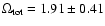 for the TONRY data set,
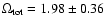 for the RIESS(w/o HST) data set and
 for the RIESS data set.
Alternatively, one can also compute the probability
for the RIESS data set.
Alternatively, one can also compute the probability
 of obtaining
,
which is
found to be
of obtaining
,
which is
found to be
 for the TONRY data set,
 for the RIESS(w/o HST) data set and
 for the RIESS data set.
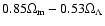
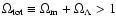
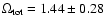
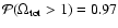
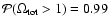
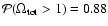
Although there is a general consensus that the
"concordance'' cosmological model
has
for the RIESS data set.
Although there is a general consensus that the
"concordance'' cosmological model
has
 ,
one should keep in mind that as
far as supernova data alone is
concerned, it is highly probable that
- in particular,
the probability
is quite high (0.97)
when the recent HST data points are not included in the analysis.
The presence
of 14 new HST points
at redshifts around 1 to 1.6 makes sure that the probability
of obtaining
is somewhat lower (<0.9).
,
one should keep in mind that as
far as supernova data alone is
concerned, it is highly probable that
- in particular,
the probability
is quite high (0.97)
when the recent HST data points are not included in the analysis.
The presence
of 14 new HST points
at redshifts around 1 to 1.6 makes sure that the probability
of obtaining
is somewhat lower (<0.9).
![\begin{figure}
\par\includegraphics[angle=270,width=16cm,clip]{1168fig5.ps}
\end{figure}](/articles/aa/full/2005/03/aa1168/Timg88.gif) |
Figure 5:
Confidence region
ellipses in the
plane for models with
non-relativistic matter and a cosmological constant,
allowing for possibly different
for the different redshift subsamples.
It is assumed that supernovae at z < 0.34 have
 ,
while those at z > 0.34 have ,
while those at z > 0.34 have
 .
The ellipses corresponding to the
68, 90 and 99 per cent confidence regions are shown.
The confidence regions are obtained after marginalizing
over
.
The dashed line corresponds to the flat
model
.
The dot-dashed line denotes the models having zero deceleration
at the present epoch
(i.e., q0 = 0), with the region below this line representing
the non-accelerating models.
The left, middle and right panels show data points for the data sets RIESS, RIESS(w/o HST) and TONRY respectively.
The values of the best-fit parameters, with
1 errors are indicated in the respective panels. .
The ellipses corresponding to the
68, 90 and 99 per cent confidence regions are shown.
The confidence regions are obtained after marginalizing
over
.
The dashed line corresponds to the flat
model
.
The dot-dashed line denotes the models having zero deceleration
at the present epoch
(i.e., q0 = 0), with the region below this line representing
the non-accelerating models.
The left, middle and right panels show data points for the data sets RIESS, RIESS(w/o HST) and TONRY respectively.
The values of the best-fit parameters, with
1 errors are indicated in the respective panels. |
| Open with DEXTER |
Finally, we comment on the interplay between high and low
redshift data for non-flat models. Just as in the case of the flat models,
we divide the full data set into low (z < 0.34) and high
(z > 0.34) redshift subsets, and repeat the best-fit analysis.
The resulting confidence contours are shown
in the middle and right panels of Fig. 4, which should
be compared with panels (a) and (e) of Fig. 7 in Paper I.
One can see that
it is not possible to rule out the SCDM model using
only high redshift data points when there are large
uncertainties in
,
which agrees with what we
concluded in Paper I.
It is also clear that, like in Paper I,
the low redshift data for the TONRY data set cannot be used to discriminate
between cosmological models effectively because of large errors on the data.
However, the situation is quite different for the RIESS(w/o HST) and RIESS data sets. As we discussed before, the reduced uncertainties in these
data sets have made it possible to rule out the SCDM model using
low redshift data only. It is thus very important to have more data points
at low redshifts (with less distance uncertainties) so as to
conclude about the existence of accelerating phase of the universe,
irrespective of evolutionary effects in absolute luminosities of supernovae.
We also note, as we did for flat models, that the
best-fit value of
are substantially
different for the two subsets (as indicated in the middle and right-hand
panels of Fig. 4) with
the difference being most for the TONRY data set
and least for the RIESS data set.
We can thus take our analysis
one step further by fitting supernovae from all redshifts
while allowing for possibly different
for the different redshift samples. To be precise,
we assume that supernovae at lower redshifts
z < 0.34 have
,
while those at higher redshifts have
.
Given these, we can fit the data with four parameters
and then marginalize over
and
.
The resulting confidence regions
in the
plane are shown in
Fig. 5
for the three data sets.
![\begin{figure}
\par\includegraphics[angle=270,width=15cm,clip]{1168fig6.ps}
\end{figure}](/articles/aa/full/2005/03/aa1168/Timg89.gif) |
Figure 6:
Confidence region
ellipses in the
w 0 - w1 plane for flat models with
a fixed value of
,
as indicated
in the frames.
The confidence regions are obtained after marginalizing over
.
The
ellipses corresponding to the 68, 90 and 99 per cent confidence regions are shown.
The square point denotes the equation of state
for a universe with a non-evolving dark energy component (the
cosmological constant). The unbroken
slanted line corresponds to the contour of
constant luminosity distance, Q(z) = constant.
The top, middle and bottom rows show data points for the data sets RIESS, RIESS(w/o HST) and TONRY respectively.
The best-fit values of the fitted parameters w0 and w1 are indicated
in the panels, alongwith the corresponding errors. |
| Open with DEXTER |
As is clear from the figure, one has quite different values for
 and
and
 for the TONRY data set, while the difference is lower for the other two
data sets. This probably indicates that the difference
in the values of
for different subsets for the
TONRY data set arises from systematic errors, which are claimed
to be reduced for the other two data sets. One requires
more work, possibly a rigorous study using Monte-Carlo simulations,
to understand this in detail.
One should also note that the
data is consistent with the
non-accelerating models
at 68 and 99 percent confidence levels
for the TONRY and RIESS data sets respectively, while they
are ruled out for the RIESS(w/o HST) data set.
for the TONRY data set, while the difference is lower for the other two
data sets. This probably indicates that the difference
in the values of
for different subsets for the
TONRY data set arises from systematic errors, which are claimed
to be reduced for the other two data sets. One requires
more work, possibly a rigorous study using Monte-Carlo simulations,
to understand this in detail.
One should also note that the
data is consistent with the
non-accelerating models
at 68 and 99 percent confidence levels
for the TONRY and RIESS data sets respectively, while they
are ruled out for the RIESS(w/o HST) data set.
Before ending this section, let us explain a subtle point in determining
and
from geometrical observations.
As has been discussed in Paper I, the only
non-trivial metric function in a Friedmann universe is the
Hubble parameter H(z) (besides the curvature of the spatial
part of the metric), hence, it is not possible to determine the energy
densities of individual components of energy densities in the
universe from any geometrical observation.
However, the analysis in this section might give the wrong impression
that we have actually been able to determine both
and
just from geometrical observations.
The point to note that we have made a crucial additional
assumption that the
universe is dominated by non-relativistic matter and a cosmological
constant, with known equations of state. Once this assumption
about the equations of state is made, it allows us to determine
the energy densities of the individual components.
On the other hand, if, for example,
we generalize the composition of the universe from a simple cosmological
constant to a more general dark energy with unknown equation of state, it
will turn out that the constraints will become much weaker. We shall take
up this issue in the next section.
3 Constraints on evolving dark energy
As we have discussed in Paper I, the supernova data can be used for
constraining the equation of state of the dark energy.
In this section, we shall examine the possibility of
constraining wX(z) by comparing theoretical
models with supernova observations.
As done in Paper I, we parametrize the function wX(z) in
terms of two parameters w0 and w1:
 |
(16) |
and constrain these parameters from observations. We shall
confine our analyses to flat models in this section
(keeping in mind that the supernova data favours a
universe with
when
w0 = -1, w1=0).
If we assume wX does not evolve with time (w1 = 0), then
a simple best-fit analysis for RIESS data set shows that for a flat model with
 and
and
 (the best-fit
parameters for flat models, obtained in the previous section),
the best-fit value of w0 is
(the best-fit
parameters for flat models, obtained in the previous section),
the best-fit value of w0 is
 (which is nothing but the
conventional cosmological constant). The data, as before in Paper I,
clearly rules out
models with
w0 > -1/3 at a high
confidence level, thereby supporting the existence of
a dark energy component with negative pressure.
(which is nothing but the
conventional cosmological constant). The data, as before in Paper I,
clearly rules out
models with
w0 > -1/3 at a high
confidence level, thereby supporting the existence of
a dark energy component with negative pressure.
One can extend the analysis to find the constraints in the
w0 - w1 plane.
As before, we limit our analysis to a flat universe. Ideally, one should
fit all the four parameters
 ,
and
then marginalize over
and
to obtain the
constraints on wX.
However, if we put a uniform prior on
in the whole range, then
it turns out that it is impossible to get any sensible constraints
on w0 and w1. Furthermore, we would like to present the results in
such a manner so that one can see how the uncertainty in
affects the constraints on wX.
Keeping this in mind, we fix the value of
to 0.2, 0.3 and 0.4 (which are typical range of values determined by
other observations, like the LSS surveys, and are independent
of the nature of the dark energy; Tegmark et al. 2004a; Pope et al. 2004; Tegmark et al. 2004b), and
marginalize only over
.
,
and
then marginalize over
and
to obtain the
constraints on wX.
However, if we put a uniform prior on
in the whole range, then
it turns out that it is impossible to get any sensible constraints
on w0 and w1. Furthermore, we would like to present the results in
such a manner so that one can see how the uncertainty in
affects the constraints on wX.
Keeping this in mind, we fix the value of
to 0.2, 0.3 and 0.4 (which are typical range of values determined by
other observations, like the LSS surveys, and are independent
of the nature of the dark energy; Tegmark et al. 2004a; Pope et al. 2004; Tegmark et al. 2004b), and
marginalize only over
.
![\begin{figure}
\par\includegraphics[angle=270,width=16cm,clip]{1168fig7.ps}
\end{figure}](/articles/aa/full/2005/03/aa1168/Timg97.gif) |
Figure 7:
Confidence region
ellipses in the
plane for models with
non-relativistic matter and a cosmological constant for
different selection criteria based on extinction for the TONRY data set.
The ellipses corresponding to the
68, 90 and 99 per cent confidence regions are shown.
The confidence regions are obtained after marginalizing
over
.
The dashed line corresponds to the flat
model
.
The left panel shows results when only those points with
 are included, the middle panel
considers only points which have
are included, the middle panel
considers only points which have
 ,
while the
right panel includes all the points irrespective of the value
of .
The values of the best-fit parameters, with
1 errors are indicated in the respective panels. ,
while the
right panel includes all the points irrespective of the value
of .
The values of the best-fit parameters, with
1 errors are indicated in the respective panels.
|
| Open with DEXTER |
The
confidence contours for the three data sets are shown in Fig. 6,
which can be compared with Fig. 8 of Paper I.
The square point denotes the equation of state
for a universe with a non-evolving dark energy component (the
cosmological constant).
The main points revealed by this figure are:
(i) the confidence contours are quite
sensitive to the value of
used, thus
confirming the fact (which was mentioned in Paper I) that it
is difficult to constrain wX with uncertainties
in
.
For example, in the TONRY data set,
we see that non-accelerating models
with
w0 < -1/3 are ruled out with a high degree
of confidence for low values of
,
while it is possible to
accommodate them for
 .
We have elaborated this point in Paper I by studying the
sensitivity of Q(z) to w0 and w1 with varying
.
(ii) The shape of the confidence
contours clearly indicates that the data is not as sensitive to w1 as compared to w0. We stressed in Paper I that
this has nothing to do with the supernova data as such. Essentially,
the supernova observations measure Q(z) and it turns out that Q(z) is
comparatively
insensitive to w1.
(iii) The best-fit values for all the
three data sets strongly favour models with w0 < -1, which
indicate the possibility of exotic forms of energy densities -
possibly scalar fields
with negative kinetic energies (such models are explored, for example, in
Caldwell 2002; Hannestad & Mörtsell 2002; Carroll et al. 2003; Caldwell et al. 2003; Melchiorri et al. 2003; Singh et al. 2003; Johri 2004; Stefancic 2004; Sami & Toporensky 2004; Li & Hao 2004; Hao & Li 2004; Szydlowski et al. 2004; Piao & Zhang 2004). However,
one should note that all the three data sets are still quite consistent
with the standard cosmological constant
(
w0=-1,w1=0)
at 99 per cent confidence level for relatively
higher values of
.
One still requires data sets of
better qualities
to settle this issue.
(iv) The inclusion of the new HST data points (RIESS data set) have resulted
in drastic decrease in the best-fit
value of w1 (from 5.92 to 3.31 for
.
We have elaborated this point in Paper I by studying the
sensitivity of Q(z) to w0 and w1 with varying
.
(ii) The shape of the confidence
contours clearly indicates that the data is not as sensitive to w1 as compared to w0. We stressed in Paper I that
this has nothing to do with the supernova data as such. Essentially,
the supernova observations measure Q(z) and it turns out that Q(z) is
comparatively
insensitive to w1.
(iii) The best-fit values for all the
three data sets strongly favour models with w0 < -1, which
indicate the possibility of exotic forms of energy densities -
possibly scalar fields
with negative kinetic energies (such models are explored, for example, in
Caldwell 2002; Hannestad & Mörtsell 2002; Carroll et al. 2003; Caldwell et al. 2003; Melchiorri et al. 2003; Singh et al. 2003; Johri 2004; Stefancic 2004; Sami & Toporensky 2004; Li & Hao 2004; Hao & Li 2004; Szydlowski et al. 2004; Piao & Zhang 2004). However,
one should note that all the three data sets are still quite consistent
with the standard cosmological constant
(
w0=-1,w1=0)
at 99 per cent confidence level for relatively
higher values of
.
One still requires data sets of
better qualities
to settle this issue.
(iv) The inclusion of the new HST data points (RIESS data set) have resulted
in drastic decrease in the best-fit
value of w1 (from 5.92 to 3.31 for
 ),
implying less rapid variation
of wX(z).
),
implying less rapid variation
of wX(z).
We have reanalyzed the supernova data with the currently available data
points and constrained various parameters related to
general cosmological models and dark energy.
We would like to mention that our analysis ignores the effects of correlation
and other systematics present in the data.
The main aim of the work has been to focus on some important theoretical issues which
are not adequately stressed in the literature.
We have used three compiled
and available data sets, which are called TONRY (194 points),
RIESS(w/o HST) (142 points) and RIESS (156 points). The RIESS(w/o HST) is
obtained from the TONRY data set by discarding points with
large uncertainties and by reducing calibration errors, while the
RIESS data set is obtained by adding the recent points from HST to the
RIESS(w/o HST) set. The analysis
is an extension to what was performed in Paper I with a small subset
of data points.
In particular, we have critically compared the estimated values of
cosmological parameters from the three data sets.
While the errors on the parameter estimation
have come down significantly with all the data sets, we find that
there some crucial differences between the data sets.
We summarize the key results once more:
It has been well known that the supernova data
rule out the flat and open matter-dominated models
with a high degree of confidence
(Perlmutter et al. 1999; Riess 2000; Riess et al. 1998). However, for the TONRY and
RIESS(w/o HST) data sets, we find that the data
favours a model with
(with probability  )
and
is in mild
disagreement with the "concordance'' flat models
with cosmological constant.
This disagreement seem to be less (the
probability of obtaining models with
being
)
and
is in mild
disagreement with the "concordance'' flat models
with cosmological constant.
This disagreement seem to be less (the
probability of obtaining models with
being
 )
for the RIESS data set,
which includes the
new HST points in the redshift range
1 < z < 1.6,
)
for the RIESS data set,
which includes the
new HST points in the redshift range
1 < z < 1.6,
The supernova data on the whole
rules out non-accelerating models with very high confidence
level.
However, it is interesting
to note that if we divide the TONRY data set
into high and low redshift subsets,
neither
of the subsets are able to rule out the non-accelerating models.
In particular, the low redshift data points are consistent with the
non-accelerating models because of large errors on the data.
This keeps open the possibility that the evolutionary effects
in the absolute luminosities of supernovae might make
the entire data set consistent with SCDM model.
The situation is quite different for the RIESS(w/o HST) and RIESS data sets,
where points with large errors are discarded.
The low redshift data
alone seem to rule out the SCDM model with high degree of confidence.
This means that unless the absolute luminosities of supernovae
evolve rapidly with redshift,
it might be difficult for the data set to be consistent
with the SCDM model. In other words, the RIESS(w/o HST) and RIESS data sets
establish the presence of the accelerating phase of the universe
regardless of the evolutionary effects.
The key issue regarding dark energy is
to determine the evolution of its equation of
state, wX. We find
that although one can constrain the current
value of wX quite well, it
is comparatively difficult
to determine the
evolution of wX. The situation
is further worsened when we take the uncertainties in
into account.
The supernova data mildly favours a dark energy equation of state
with its present best-fit value less than -1 which will require more exotic forms of matter (possibly with
negative kinetic energy). However, one should keep in mind that
the
data is still consistent with the
standard cosmological constant at 99 per cent confidence level.
The analysis of different subsamples of the supernova data set
is important in determining the effect of evolution.
In this work, we have taken the simple approach
of dividing the data roughly around the epoch where the
universe might have transited from a decelerating to an
accelerating phase, and checked whether the data can be made
consistent with the non-accelerating models. In future, it
would be interesting to divide the data based on the nature of
supernova searches. For example, one can divide the data into
three redshift splits: z < 0.1,
0.2 < z < 0.8 and z > 0.8,
which roughly correspond to supernovae discovered
in shallow searches, ground-based deep searches, and space-based deep
searches. It would be interesting to check the cosmological constraints
with such a divide.
Acknowledgements
We thank Alex Kim for extensive
comments which significantly improved the paper.
Since there is considerable uncertainty
in determining the host extinction and reddening, we have considered
only those supernova which have extinction
for the TONRY
data set.
It would be interesting to see how this selection criterion affects
our determination of cosmological parameters. In particular, one should
keep in mind that the high-redshift supernovae
observed from the ground could have large
uncertainty in their color and hence statistically will often have
measured
even if they have no extinction.
To check how this affects the cosmological parameters, we concentrate
on the cosmological models with non-relativistic matter and
a cosmological constant, and find the constraints
in the
plane. We consider three
cases, namely, (i) the usual one where we exclude all the data points
with
,
(ii) the one with a stricter selection criterion where
we exclude points with
 and finally (iii) we include all
the points irrespective of the extinction. The results for the
three cases are plotted in Fig. 7.
It is clear from the figure that the exclusion of points
based on their extinction have little effect on the
determination of the cosmological parameters, at least for the
TONRY data set. The cosmological parameters agree within 1 errors
for the three different selection criteria.
and finally (iii) we include all
the points irrespective of the extinction. The results for the
three cases are plotted in Fig. 7.
It is clear from the figure that the exclusion of points
based on their extinction have little effect on the
determination of the cosmological parameters, at least for the
TONRY data set. The cosmological parameters agree within 1 errors
for the three different selection criteria.
- Alam, U., Sahni, V.,
& Starobinsky, A. A. 2004, JCAP, 0406, 008 [NASA ADS]
- Albrecht, A., &
Skordis, C. 2000, Phys. Rev. Lett., 84, 2076 [NASA ADS] [CrossRef]
- Alcaniz,
J. S. 2004, Phys. Rev. D, 69, 083521 [NASA ADS] [CrossRef]
- Alcaniz, J. S., &
Pires, N. 2004, Phys. Rev. D, 70, 047303 [NASA ADS] [CrossRef]
- Astier, P. 2000,
Preprint [arXiv:astro-ph/0008306]
- Bagla, J. S.,
Jassal, H. K., & Padmanabhan, T. 2003, Phys. Rev. D, 67,
063504 [NASA ADS] [CrossRef]
- Barreiro, T., Copeland,
E. J., & Nunes, N. J. 2000, Phys. Rev. D, 61,
127301 [NASA ADS] [CrossRef]
- Barris, B. J., Tonry, J.,
Blondin, S., et al. 2004, ApJ, 602, 571 [NASA ADS] [CrossRef]
- Bertolami, O.
2004, Preprint [arXiv:astro-ph/0403310]
- Bertolami, O., Sen,
A. A., Sen, S., & Silva, P. T. 2004, MNRAS, 353,
329 [NASA ADS] [CrossRef]
- Bilic, N., Tupper,
G. B., & Viollier, R. D. 2002, Phys. Lett. B, 535,
17 [NASA ADS] [CrossRef]
- Brax, P., & Martin, J.
1999, Phys. Lett. B, 468, 40 [NASA ADS] [CrossRef] [MathSciNet]
- Brax, P., & Martin,
J. 2000, Phys. Rev., D, 61, 103502
- Caldwell,
R. R. 2002, Phys. Lett. B, 545, 23 [NASA ADS] [CrossRef] (In the text)
- Caldwell, R. R.,
Kamionkowski, M., & Weinberg, N. N. 2003, Phys. Rev.
Lett., 91, 071301 [NASA ADS] [CrossRef] (In the text)
- Caresia, P., Matarrese,
S., & Moscardini, L. 2004, ApJ, 605, 21 [NASA ADS] [CrossRef]
- Carroll, S. M.,
Hoffman, M., & Trodden, M. 2003, Phys. Rev. D, 68, 023509 [NASA ADS] [CrossRef] (In the text)
- Chae, K.-H., Chen, G.,
Ratra, B., & Lee, D.-W. 2004, ApJ, 607, L71 [NASA ADS] [CrossRef]
- Corasaniti, P. S.,
& Copeland, E. J. 2002, Phys. Rev. D, 65, 043004 [NASA ADS] [CrossRef]
- Daly, R. A., &
Djorgovski, S. G. 2003, ApJ, 597, 9 [NASA ADS] [CrossRef] (In the text)
- Dev, A., Jain, D., &
Alcaniz, J. S. 2004, A&A, 417, 847 [EDP Sciences] [NASA ADS] [CrossRef]
- Fairbairn, M., &
Tytgat, M. H. G. 2002, Phys. Lett. B, 546, 1 [NASA ADS] [CrossRef]
- Feinstein, A.
2002, Phys. Rev. D, 66, 063511 [NASA ADS] [CrossRef]
- Ferreira, P. G., &
Joyce, M. 1998, Phys. Rev. D, 58, 023503 [NASA ADS] [CrossRef]
- Frieman, J. A.,
Hill, C. T., Stebbins, A., & Waga, I. 1995, Phys. Rev.
Lett., 75, 2077 [NASA ADS] [CrossRef]
- Frolov, A., Kofman, L.,
& Starobinsky, A. A. 2002, Phys. Lett. B, 545, 8 [NASA ADS] [CrossRef]
- Garnavich, P. M., Jha, S.,
Challis, P., et al. 1998, ApJ, 509, 74 [NASA ADS] [CrossRef]
- Gerke, B. F., &
Efstathiou, G. 2002, MNRAS, 335, 33 [NASA ADS] [CrossRef]
- Gibbons,
G. W. 2002, Phys. Lett. B, 537, 1 [NASA ADS] [CrossRef] [MathSciNet]
- Goliath, M.,
Amanullah, R., Astier, P., Goobar, A., & Pain, R. 2001,
Preprint [arXiv:astro-ph/0104009]
- Gong, Y.-G. 2004,
Preprint [arXiv:astro-ph/0401207]
- Gong, Y.-g., & Chen,
X.-M. 2004, Preprint [arXiv:gr-qc/0402031]
- Gong, Y.-G., Chen, X.-M.,
& Duan, C.-K. 2004, Mod. Phys. Lett. A, 19, 1933 [NASA ADS]
- Gong, Y.-G., & Duan,
C.-K. 2004, MNRAS, 352, 847 [NASA ADS] [CrossRef]
- Goobar, A., Mörtsell, E.,
Amanullah, R., et al. 2002a, A&A, 392, 757 [EDP Sciences] [NASA ADS] [CrossRef]
- Goobar, A.,
Mörtsell, E., Amanullah, R., & Nugent, P. 2002b, A&A,
393, 25 [EDP Sciences] [NASA ADS] [CrossRef]
- Goobar, A., &
Perlmutter, S. 1995, ApJ, 450, 14 [NASA ADS] [CrossRef] (In the text)
- Hannestad, S., &
Mörtsell, E. 2002, Phys. Rev. D, 66, 063508 [NASA ADS] [CrossRef] (In the text)
- Hao, J.-g., & Li, X.-z.
2004, Preprint [arXiv:astro-ph/0404154]
(In the text)
- Huterer, D., Kim, A.,
Krauss, L. M., & Broderick, T. 2004, Preprint
[arXiv:astro-ph/0402002]
- Johri, V. B.
2004, Phys. Rev. D, 70, 041303 [NASA ADS] [CrossRef] (In the text)
- Kim, A. G.,
Linder, E. V., Miquel, R., & Mostek, N. 2004, MNRAS, 347,
909 [NASA ADS] [CrossRef]
- Knop, R. A., Aldering, G.,
Amanullah, R., et al. 2003, ApJ, 598, 102 [NASA ADS] [CrossRef]
- Kujat, J., Linn,
A. M., Scherrer, R. J., & Weinberg, D. H. 2002,
ApJ, 572, 1 [NASA ADS] [CrossRef]
- Leibundgut, B. 2001, ARA&A, 39, 67 [NASA ADS]
- Li, X.-Z., & Hao, J.-G.
2004, Phys. Rev. D, 69, 107303 [NASA ADS] [CrossRef] (In the text)
- Lima, J. A. S.,
& Alcaniz, J. S. 2004, Phys. Lett. B, 600, 191 [NASA ADS] [CrossRef]
- Linder, E. V.
2004, Preprint [arXiv:astro-ph/0406186]
- Linder, E. V., & Huterer,
D. 2003, Phys. Rev. D, 67, 081303 [NASA ADS] [CrossRef]
- Linder, E. V., &
Jenkins, A. 2003, MNRAS, 346, 573 [NASA ADS] [CrossRef]
- Maor, I., Brustein, R.,
McMahon, J., & Steinhardt, P. J. 2002, Phys. Rev. D, 65,
123003 [NASA ADS] [CrossRef]
- McInnes, B. 2004,
JHEP, 04, 036 [NASA ADS] [CrossRef] [MathSciNet]
- Melchiorri, A.,
Mersini, L., Ödman, C. J., & Trodden, M. 2003, Phys.
Rev. D, 68, 043509 [NASA ADS] [CrossRef] (In the text)
- Minty, E. M.,
Heavens, A. F., & Hawkins, M. R. S. 2002, MNRAS,
330, 378 [NASA ADS] [CrossRef]
- Mukohyama, S.
2002, Phys. Rev. D, 66, 024009 [NASA ADS] [CrossRef] [MathSciNet]
- Nesseris, S., &
Perivolaropoulos, L. 2004, Phys. Rev. D, 70, 043531 [NASA ADS] [CrossRef]
- Novello, M.,
Perez Bergliaffa, S. E., & Salim, J. 2003,
Preprint[arXiv:astro-ph/0312093]
- Padmanabhan, T. 2002, Phys. Rev. D, 66, 021301 [NASA ADS] [CrossRef]
- Padmanabhan, T. 2003, Phys. Rept., 380, 235 [NASA ADS] [CrossRef] [MathSciNet]
- Padmanabhan, T., &
Choudhury, T. R. 2002, Phys. Rev. D, 66, 081301 [NASA ADS] [CrossRef]
- Padmanabhan, T., &
Choudhury, T. R. 2003, MNRAS, 344, 823 [NASA ADS] [CrossRef] (Paper I)
(In the text)
- Peebles, P. J., &
Ratra, B. 2003, Rev. Mod. Phys., 75, 559 [NASA ADS] [CrossRef] [MathSciNet] (In the text)
- Peebles,
P. J. E., & Ratra, B. 1988, ApJ, 325, L17 [NASA ADS] [CrossRef]
- Perlmutter, S., Aldering, G.,
Goldhaber, G., et al. 1999, ApJ, 517, 565 [NASA ADS] [CrossRef]
- Perlmutter, S., Gabi, S.,
Goldhaber, G., et al. 1997, ApJ, 483, 565 [NASA ADS] [CrossRef]
- Perlmutter, S., &
Schmidt, B. P. 2003, Lect. Notes Phys. (Berlin: Springer
Verlag), 598, 195 [NASA ADS]
- Phillips, M. M., Lira, P.,
Suntzeff, N. B., et al. 1999, AJ, 118, 1766 [NASA ADS] [CrossRef]
- Piao, Y.-S., & Zhang,
Y.-Z. 2004, Phys. Rev. D, 70, 063513 [NASA ADS] [CrossRef] (In the text)
- Podariu, S., Nugent, P.,
& Ratra, B. 2001, ApJ, 553, 39 [NASA ADS] [CrossRef]
- Pope, A. C., Matsubara, T.,
Szalay, A. S., et al. 2004, ApJ, 607, 655 [NASA ADS] [CrossRef]
- Ratra, B., & Peebles,
P. J. E. 1988, Phys. Rev. D, 37, 3406 [NASA ADS] [CrossRef]
- Riess, A. G.
2000, PASP, 112, 1284 [NASA ADS] [CrossRef]
- Riess, A. G., Filippenko,
A. V., Challis, P., et al. 1998, AJ, 116, 1009 [NASA ADS] [CrossRef]
- Riess, A. G., Press,
W. H., & Kirshner, R. P. 1996, ApJ, 473, 88 [NASA ADS] [CrossRef]
- Riess, A. G., Strolger, L.,
Tonry, J., et al. 2004, ApJ, 607, 665 [NASA ADS] [CrossRef]
- Rowan-Robinson, M. 2002, MNRAS, 332, 352 [NASA ADS] [CrossRef]
- Sahni, V., &
Starobinsky, A. A. 2000, Int. J. Mod. Phys. D, 9, 373 [NASA ADS] [CrossRef] (In the text)
- Saini, T. D.,
Raychaudhury, S., Sahni, V., & Starobinsky, A. A. 2000,
Phys. Rev. Lett., 85, 1162 [NASA ADS] [CrossRef]
- Sami, M., & Toporensky,
A. 2004, Mod. Phys. Lett. A, 19, 1509 [NASA ADS] (In the text)
- Shiu, G., & Wasserman,
I. 2002, Phys. Lett. B, 541, 6 [NASA ADS] [CrossRef]
- Singh, P., Sami, M.,
& Dadhich, N. 2003, Phys. Rev. D, 68, 023522 [NASA ADS] [CrossRef] (In the text)
- Spergel, D. N., Verde, L.,
Peiris, H. V., et al. 2003, ApJS, 148, 175 [NASA ADS] [CrossRef]
- Stefancic, H.
2004, Eur. Phys. J. C, 36, 523 [EDP Sciences] [NASA ADS] (In the text)
- Szydlowski, M., &
Czaja, W. 2004, Preprint [arXiv:astro-ph/0402510]
- Szydlowski, M., Czaja,
W., & Krawiec, A. 2004, Preprint
[arXiv:astro-ph/0401293]
(In the text)
- Tegmark, M., Blanton, M. R.,
Strauss, M. A., et al. 2004a, ApJ, 606, 702 [NASA ADS] [CrossRef]
- Tegmark, M., Strauss, M. A.,
Blanton, M. R., et al. 2004b, Phys. Rev. D, 69,
103501 [NASA ADS] [CrossRef]
- Tonry, J. L., Schmidt,
B. P., Barris, B., et al. 2003, ApJ, 594, 1 [NASA ADS] [CrossRef]
- Trentham, N.
2001, MNRAS, 326, 1328 [NASA ADS]
- Urena-Lopez, L. A.,
& Matos, T. 2000, Phys. Rev. D, 62, 081302 [NASA ADS] [CrossRef]
- Visser, M. 2004,
Classical Quantum Gravity, 21, 2603 [NASA ADS] [CrossRef] [MathSciNet]
- Wang, Y. 2004, Preprint
[arXiv:astro-ph/0406635]
- Wang, Y., & Garnavich,
P. M. 2001, ApJ, 552, 445 [NASA ADS] [CrossRef]
- Wang, Y., & Lovelace,
G. 2001, ApJ, 562, L115 [NASA ADS]
- Wang, Y., & Mukherjee,
P. 2004, ApJ, 606, 654 [NASA ADS] [CrossRef]
- Wang, Y., & Tegmark, M.
2004, Phys. Rev. Lett., 92, 241302 [NASA ADS] [CrossRef]
- Weller, J., & Albrecht,
A. 2001, Phys. Rev. Lett., 86, 1939 [NASA ADS] [CrossRef]
- Weller, J., & Albrecht,
A. 2002, Phys. Rev. D, 65, 103512 [NASA ADS] [CrossRef]
- Wetterich, C.
1988, Nucl. Phys., B302, 668 [NASA ADS] [CrossRef]
- Zhu, Z.-H., & Fujimoto,
M.-K. 2003, ApJ, 585, 52 [NASA ADS] [CrossRef]
- Zhu, Z.-H., Fujimoto,
M.-K., & He, X.-T. 2004, A&A, 417, 833 [EDP Sciences] [NASA ADS] [CrossRef]
- Zlatev, I., Wang, L.-M.,
& Steinhardt, P. J. 1999, Phys. Rev. Lett., 82, 896 [NASA ADS] [CrossRef]
Copyright ESO 2005
![\begin{figure}
\par\includegraphics[angle=270,width=8cm,clip]{1168fig1.ps}
\end{figure}](/articles/aa/full/2005/03/aa1168/img48.gif)
![\begin{figure}
\par\includegraphics[angle=270,width=17cm,clip]{1168fig2.ps}
\end{figure}](/articles/aa/full/2005/03/aa1168/img50.gif)
![\begin{figure}
\par\includegraphics[angle=270,width=15cm,clip]{1168fig3.ps}
\end{figure}](/articles/aa/full/2005/03/aa1168/img51.gif)
![\begin{figure}
\par\includegraphics[angle=270,width=16.2cm,clip]{1168fig4.ps}
\end{figure}](/articles/aa/full/2005/03/aa1168/img70.gif)
![\begin{figure}
\par\includegraphics[angle=270,width=16cm,clip]{1168fig5.ps}
\end{figure}](/articles/aa/full/2005/03/aa1168/img88.gif)
![\begin{figure}
\par\includegraphics[angle=270,width=15cm,clip]{1168fig6.ps}
\end{figure}](/articles/aa/full/2005/03/aa1168/img89.gif)
![\begin{figure}
\par\includegraphics[angle=270,width=16cm,clip]{1168fig7.ps}
\end{figure}](/articles/aa/full/2005/03/aa1168/img97.gif)