A&A 418, 639-648 (2004)
DOI: 10.1051/0004-6361:20040090
C. Aerts1 - H. J. G. L. M. Lamers2,3 - G. Molenberghs4
1 - Institute of Astronomy, Catholic University of Leuven,
Celestijnenlaan 200 B, 3001 Leuven, Belgium
2 - Astronomical Institute,
Utrecht University, PO Box 80000, 3508 TA Utrecht, The Netherlands
3 - SRON Laboratory, for Space Research, Sorbonnelaan 2, 3584 CA Utrecht, The
Netherlands
4 -
Center for Statistics, Limburgs Universitair Centrum,
Universitaire Campus, Building D, 3590 Diepenbeek, Belgium
Received 31 March 2003 / Accepted 10 January 2004
Abstract
We investigate the effect of rotation on the maximum mass-loss rate
due to an optically-thin radiatively-driven wind according to a formalism which
takes into account the possible presence of any instability at the base of the
wind that might increase the mass-loss rate. We include the Von Zeipel effect
and the oblateness of the star in our calculations. We determine the maximum
surface-integrated mass that can be lost from a star by line driving as a
function of rotation for a number of relevant stellar models of massive OB stars
with luminosities in the range of
![]() .
We also
determine the corresponding maximum loss of angular momentum. We find that
rotation increases the maximum mass-loss rate by a moderate factor for stars far
from the Eddington limit as long as the ratio of equatorial to critical velocity
remains below 0.7. For higher ratios, however, the temperature, flux and
Eddington factor distributions change considerably over the stellar surface such
that extreme mass loss is induced. Stars close to the Eddington-Gamma limit
suffer extreme mass loss already for a low equatorial rotation velocity. We
compare the maximum mass-loss rates as a function of rotation velocity with
other predicted relations available in the literature which do not take into
account possible instabilities at the stellar surface and we find that the
inclusion thereof leads to extreme mass loss at much lower rotation rates. We
present a scaling law to predict maximum mass-loss rates. Finally, we provide a
mass-loss model for the LBV
.
We also
determine the corresponding maximum loss of angular momentum. We find that
rotation increases the maximum mass-loss rate by a moderate factor for stars far
from the Eddington limit as long as the ratio of equatorial to critical velocity
remains below 0.7. For higher ratios, however, the temperature, flux and
Eddington factor distributions change considerably over the stellar surface such
that extreme mass loss is induced. Stars close to the Eddington-Gamma limit
suffer extreme mass loss already for a low equatorial rotation velocity. We
compare the maximum mass-loss rates as a function of rotation velocity with
other predicted relations available in the literature which do not take into
account possible instabilities at the stellar surface and we find that the
inclusion thereof leads to extreme mass loss at much lower rotation rates. We
present a scaling law to predict maximum mass-loss rates. Finally, we provide a
mass-loss model for the LBV ![]() Carinae that is able to explain the large
observed current mass-loss rate of
Carinae that is able to explain the large
observed current mass-loss rate of ![]()
![]() yr-1 but that
leads to too low wind velocities compared to those derived from observations.
yr-1 but that
leads to too low wind velocities compared to those derived from observations.
Key words: stars: early-type - stars: mass-loss - stars: winds, outflows - stars:
evolution - methods: statistical - stars: individual: ![]() Car
Car
Rapidly rotating massive stars may suffer mass-loss rates that are considerably higher than those of non-rotating stars. Stellar evolution calculations indeed show that rapidly rotating stars must lose a large fraction of their mass in a relatively short time (Langer 1998). For the calculation of the evolution of rotating stars Langer (1998) used an expression for the mass-loss rate of rotating stars, based on an interpolation and extrapolation of the models from Friend & Abbott's (1986) early study of rotating line-driven winds. This expression predicts that the mass-loss rate becomes extremely high when the star rotates close to critical velocity. This result was criticized by Glatzel (1998) and by Owocki et al. (1998), who find that the mass-loss rates at critical velocity do not differ too much from those of a non-rotating star.
Maeder & Meynet (2000) propose a new scaling law for the increase of mass loss
with the rotation velocity by taking into account the Von Zeipel effect and the
oblateness of the star. This law depends on the Eddington factor ![]() ,
the
CAK line-force parameter
,
the
CAK line-force parameter ![]() (Castor et al. 1975, hereafter called CAK) and
the critical velocity. It predicts a finite mass-loss rate close to critical
velocity for stars sufficiently far from the Eddington limit, i.e. for
(Castor et al. 1975, hereafter called CAK) and
the critical velocity. It predicts a finite mass-loss rate close to critical
velocity for stars sufficiently far from the Eddington limit, i.e. for ![]() roughly below 0.3. For higher values of
roughly below 0.3. For higher values of ![]() ,
however, extreme mass loss is
derived. Our current study elaborates further on this by including any kind of
instability at the base of the stellar wind that might increase the mass-loss
rate. In particular, the purpose of our work is to investigate how much mass
can maximally be expelled from a rotating star by radiation pressure due to
spectral lines, by allowing for the most optimistic circumstances near the sonic
point. This work can be seen as a generalisation of Maeder & Meynet
(2000). We explicitly integrate the momentum equation for different latitudes to
find the surface-integrated maximum mass-loss as a function of rotation velocity
rather than using a scaling law for the mass loss of a non-rotating and a
rotating star. Moreover, we allow for an unspecified extra force (e.g. due to
pulsation or magnetic fields) at the stellar surface that changes the velocity
gradient at the sonic point and helps in this way in the onset of the mass loss.
,
however, extreme mass loss is
derived. Our current study elaborates further on this by including any kind of
instability at the base of the stellar wind that might increase the mass-loss
rate. In particular, the purpose of our work is to investigate how much mass
can maximally be expelled from a rotating star by radiation pressure due to
spectral lines, by allowing for the most optimistic circumstances near the sonic
point. This work can be seen as a generalisation of Maeder & Meynet
(2000). We explicitly integrate the momentum equation for different latitudes to
find the surface-integrated maximum mass-loss as a function of rotation velocity
rather than using a scaling law for the mass loss of a non-rotating and a
rotating star. Moreover, we allow for an unspecified extra force (e.g. due to
pulsation or magnetic fields) at the stellar surface that changes the velocity
gradient at the sonic point and helps in this way in the onset of the mass loss.
Very recently, Aerts & Lamers (2003, hereafter termed Paper I) presented a
formalism to derive maximum equatorial mass-loss rates
![]() of massive stars for which the wind is driven by radiation
pressure in spectral lines with finite disk correction, photon tiring and
rotation included. The latter, however, was included only for the equatorial
region. The rotation-induced decrease of the radiative flux from the poles to
the equator, called gravity darkening, as well as the oblateness of the star,
was neglected. Aerts & Lamers solved the momentum equation for different
positive values of the velocity gradient at the sonic point as boundary
condition. They then selected the highest possible mass loss for which an
outflowing wind is still obtained. Such a formalism is the most flexible one to
see how much mass can be driven by a CAK-type radiative force on spectral lines,
because an unspecified possible extra force (such as due to stellar
oscillations, magnetic fields or instabilities) at the base of the wind is
allowed for.
of massive stars for which the wind is driven by radiation
pressure in spectral lines with finite disk correction, photon tiring and
rotation included. The latter, however, was included only for the equatorial
region. The rotation-induced decrease of the radiative flux from the poles to
the equator, called gravity darkening, as well as the oblateness of the star,
was neglected. Aerts & Lamers solved the momentum equation for different
positive values of the velocity gradient at the sonic point as boundary
condition. They then selected the highest possible mass loss for which an
outflowing wind is still obtained. Such a formalism is the most flexible one to
see how much mass can be driven by a CAK-type radiative force on spectral lines,
because an unspecified possible extra force (such as due to stellar
oscillations, magnetic fields or instabilities) at the base of the wind is
allowed for.
These maximum mass-loss rates were compared with those predicted by classical self-regulating CAK wind theory and with the models including multiple scattering (Vink et al. 2000, 2001) which do not include instabilities at the base of the wind. The result of Paper I was that line driving can induce a maximum equatorial mass loss that is at most a factor 2-3 higher than the one of a self-regulated line-driven wind, in agreement with the earlier results of mass-overloaded wind solutions found in the studies by e.g. Poe et al. (1990), Owocki et al. (1994), Gayley (2000) and Feldmeier & Shlosman (2002). In this paper we investigate to what extent the Von Zeipel effect and rotational flattening changes the results obtained in Paper I, by performing the calculations for an oblate star and providing total surface-integrated maximum mass-loss rates instead of only equatorial ones. Our results can be compared with those of Pelupessy et al. (2000), who calculated line-driven mass-loss rates of rotating hot stars with oblateness, the von Zeipel effect and the proper finite disk correction factor taken into account, but who did not allow for the presence of an extra force.
The concept of the maximum mass-loss rate was introduced in Paper I because mechanisms other than radiation pressure and rotation are common among massive stars and may influence their mass loss. This will affect the evolution of the star if the resulting mass-loss rate is much higher than for self-regulated line-driven winds. As Paper I revealed the occurrence of maximum mass-loss rates which are only moderately higher than those considered up to now for (super)giants, and in view of the intense debate about the role of rotation on mass loss of massive stars (see e.g. Langer 1998; Glatzel 1998; Owocki et al. 1998; Maeder & Meynet 2000), we devote the current paper to the detailed study of the dependence of the maximum mass-loss rates, determined with the formalism of Paper I, on rotation.
The paper is organised as follows. In Sect. 2 we briefly recall the
ingredients of the formalism and the definitions used in Paper I to derive the
maximum mass-loss rates. In Sect. 3 we subsequently present the maximum
mass-loss rates as a function of the rotation velocity for a grid of stellar
models of massive stars. We do this by outward integration of the momentum
equation for different latitudes and by summing the corresponding local
mass-loss rates for all stellar latitudes. We also compare our values for the
surface-integrated maximum mass loss with those found from Langer's (1998)
empirical relation and with Maeder & Meynet's (2000) scaling law. We also
determine the maximum loss of angular momentum. We provide a maximum mass-loss
recipe derived from multiple regression of the calculated grid, i.e. for the
range
![]() in Sect. 4. An application of our mass-loss
calculations to the luminous blue variable
in Sect. 4. An application of our mass-loss
calculations to the luminous blue variable ![]() Carinae is presented in
Sect. 5. We end with a discussion in Sect. 6.
Carinae is presented in
Sect. 5. We end with a discussion in Sect. 6.
Table 1:
Stellar parameters of the 9 non-rotating models for which
the maximum mass-loss rates were determined in Paper I. The line
force parameters ![]() and k are taken from Pauldrach et al. (1986). The
critical velocity
and k are taken from Pauldrach et al. (1986). The
critical velocity
![]() is expressed in km s-1 while
is expressed in km s-1 while
![]() is expressed in cm2 g-1. The mass-loss rate is given in units of
10-6
is expressed in cm2 g-1. The mass-loss rate is given in units of
10-6 ![]() yr-1.
yr-1.
The starting point for the formalism developed in Paper I was to understand to
what extent the conservation of momentum and energy allow the occurrence of
extremely high mass loss. To do this, we adopted the most flexible
conditions possible, i.e. we allowed for an unspecified force at the base of
the stellar wind to help drive the wind. Such a force can result from stellar
oscillations or a magnetic field or any instability, i.e. phenomena that are
common in massive stars but that are not commonly included in line-driven wind
calculations yet. Under this condition, which replaces the usual singularity
and regularity condition adopted in a self-regulating wind, it was investigated
how large
![]() can become such that the momentum equation remains
solvable for a CAK-type parametrisation of the line-driving. This was done in
the approximation of a uniformly rotating star for which the deviation from
spherical symmetry of the physical stellar quantities and of the wind was
neglected. Finite disk correction and photon tiring were taken into account, as
well as a wind temperature law
can become such that the momentum equation remains
solvable for a CAK-type parametrisation of the line-driving. This was done in
the approximation of a uniformly rotating star for which the deviation from
spherical symmetry of the physical stellar quantities and of the wind was
neglected. Finite disk correction and photon tiring were taken into account, as
well as a wind temperature law
![]() with n=1. It was shown in
Paper I that the resulting mass loss depends only very weakly on n.
with n=1. It was shown in
Paper I that the resulting mass loss depends only very weakly on n.
The momentum equation was solved numerically from an assumed position of the
sonic point outwards, for increasing values of the mass-loss rate, until the
amount of wind material had increased so much that the acting forces could no
longer make it escape from the star. This condition is expressed mathematically
by allowing any positive velocity gradient at the sonic point so that there
is outflow. Since we are interested in the maximum mass-loss rate that can be
lifted out of the potential well of the star by radiation pressure on spectral
lines, we did not solve the subsonic structure of the wind. The velocity
gradient at the assumed sonic point was calculated numerically from the momentum
equation. We refer to Sect. 2 of Paper I for a detailed description of the
theory we adopt here. In Paper I we allowed the radius of the sonic point,
![]() ,
to be situated in the interval
,
to be situated in the interval
![]() .
It was shown
there that the highest equatorial mass-loss rates were obtained for a sonic
point as close as possible to the stellar surface, a well-known result from
classical wind theory. We hence fixed the sonic point at the position
.
It was shown
there that the highest equatorial mass-loss rates were obtained for a sonic
point as close as possible to the stellar surface, a well-known result from
classical wind theory. We hence fixed the sonic point at the position
![]() for all results shown in this paper.
for all results shown in this paper.
In Paper I, we selected the maximum mass-loss rate in the equatorial plane,
termed
![]() ,
out of all the physically relevant
solutions of the momentum equation for which this equation still has an
outflowing wind. The maximum velocity that occurs in the wind was defined as
,
out of all the physically relevant
solutions of the momentum equation for which this equation still has an
outflowing wind. The maximum velocity that occurs in the wind was defined as
![]() .
It was shown in Paper I that the
.
It was shown in Paper I that the
![]() -values
corresponding to
-values
corresponding to
![]() are typically a few hundred
km s-1 for all considered cases. This is much lower than the values of the
terminal velocity
are typically a few hundred
km s-1 for all considered cases. This is much lower than the values of the
terminal velocity ![]() predicted by the classical or modified CAK-models.
It was also found in Paper I that the mass-overloaded solutions at a high
percentage (>
predicted by the classical or modified CAK-models.
It was also found in Paper I that the mass-overloaded solutions at a high
percentage (>![]() of the critical rotation velocity have kinked velocity
laws, in agreement with earlier studies in the literature. In the following
section we focus entirely on the mass-loss rates so we do not list explicitly
the corresponding wind velocities, which are all of the order of a few hundred
km s-1.
of the critical rotation velocity have kinked velocity
laws, in agreement with earlier studies in the literature. In the following
section we focus entirely on the mass-loss rates so we do not list explicitly
the corresponding wind velocities, which are all of the order of a few hundred
km s-1.
We describe the mass-loss rates and angular momentum loss for stellar models
that are rotationally flattened and gravity-darkened.
The (equatorial) stellar parameters of the considered models are listed in
Table 1. They span a range of
![]() K,
at high luminosities between 105 and 106
K,
at high luminosities between 105 and 106 ![]() .
.
In Table 4 of Paper I, the equatorial maximum mass-loss rates for 9 spherical stars of different stellar parameters and for a large range of equatorial velocities, ranging from zero rotation up to the critical velocity, was presented, assuming the stars to be spherical solid rotators. The radiative acceleration was calculated for a spherical star with a homogeneously illuminated stellar disk, i.e. without gravity darkening. Under these simplifying assumptions the maximum mass-loss rates of stars rotating near critical were found to increase only with a factor 2-3 compared to those of non-rotating stars.
In reality, the radius, effective temperature, luminosity and Eddington factor
differ for different values of the co-latitute ![]() due to the rotation of
the star (we use the convention that the pole of the star corresponds with
due to the rotation of
the star (we use the convention that the pole of the star corresponds with
![]() ). To investigate the correct effect of rotation on
the overall maximum mass loss, the procedure outlined in Sect. 2 has to be
repeated for each co-latitude
). To investigate the correct effect of rotation on
the overall maximum mass loss, the procedure outlined in Sect. 2 has to be
repeated for each co-latitude ![]() and for increasing values of the
equatorial rotation velocity, instead of assuming spherical symmetry as was done
in Paper I. We first outline the basic assumptions we made for our calculations
before providing the final results.
and for increasing values of the
equatorial rotation velocity, instead of assuming spherical symmetry as was done
in Paper I. We first outline the basic assumptions we made for our calculations
before providing the final results.
![\begin{figure}
\par\rotatebox{270}{{\includegraphics[height=14cm,clip]{H4421.f1}}}
\end{figure}](/articles/aa/full/2004/17/aah4421/img43.gif) |
Figure 1:
The local radius ( upper left), local gravity ( upper right), local
effective temperature ( lower left) and local luminosity
|
| Open with DEXTER | |
The surface of an oblate rotating star has an inhomogeneous temperature and flux
distribution. We assume the Von Zeipel effect to be valid, which is a good
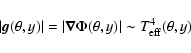
approximation for radiative stellar envelopes. The Von Zeipel theorem expresses
that the effective radiative flux from a point on a distorted star is
proportional to the local effective gravity, which can be determined by taking
into account the real shape of a uniformly rotating star. In doing so, we assume
that all the stellar mass is concentrated in the stellar centre. In that case,
the shape of the star is determined by its Roche equipotential surfaces, which
take the following dimensionless form in a co-rotating frame of reference:
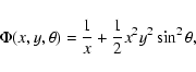 |
(1) |
![\begin{displaymath}x(\theta,y)=2\frac{\sqrt{(2+y^2)}}{\sqrt{3}\
y\sin\theta}\sin...
...ft(\frac{3\sqrt{3}\
y\sin\theta}{(2+y^2)^{3/2}}\right)}\right]
\end{displaymath}](/articles/aa/full/2004/17/aah4421/img51.gif) |
(2) |
Through the Von Zeipel theorem we are able to calculate the latitudinal
dependence of the radiative flux for a particular y:
 |
(3) |
By multiplication of x2 and
![]() ,
we also obtain the relative
local luminosity as a function of co-latitude (see Fig. 1, lower right
panel). In Fig. 1, the oblateness of the star is expressed in terms of
y, which is increased from y=0 (spherical star) to y=0.9 in steps of 0.1
for the different dotted curves in the panels.
,
we also obtain the relative
local luminosity as a function of co-latitude (see Fig. 1, lower right
panel). In Fig. 1, the oblateness of the star is expressed in terms of
y, which is increased from y=0 (spherical star) to y=0.9 in steps of 0.1
for the different dotted curves in the panels.
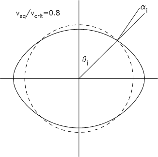 |
Figure 2:
A rotationally distorted star according to the Roche model for
|
| Open with DEXTER | |
In our model calculations we ignore any ![]() -component of the flow velocity
and we solve the momentum equation in one dimension (viz. the radial direction)
only, i.e. we solve the momentum equation (Eq. (9) of Paper I) for the values
of the relevant parameters for each co-latitude
-component of the flow velocity
and we solve the momentum equation in one dimension (viz. the radial direction)
only, i.e. we solve the momentum equation (Eq. (9) of Paper I) for the values
of the relevant parameters for each co-latitude ![]() .
We thus neglect any
wind compression due to velocity components towards the equatorial plane that
may occur, as described by Bjorkman & Cassinelli (1993). This assumption is
justified because compression merely redistributes the wind material and does
not change the total mass lost from the star, which interests us here. In this
approximation, we write the conservation of mass loss for a non-spherical
sectorial wind as
.
We thus neglect any
wind compression due to velocity components towards the equatorial plane that
may occur, as described by Bjorkman & Cassinelli (1993). This assumption is
justified because compression merely redistributes the wind material and does
not change the total mass lost from the star, which interests us here. In this
approximation, we write the conservation of mass loss for a non-spherical
sectorial wind as
| |
|||
| = | (4) |
At different values of ![]() ,
the equation to solve for the maximum mass-loss
rate at that
,
the equation to solve for the maximum mass-loss
rate at that ![]() differs because the local luminosity, the local radius and
the local effective temperature change for each co-latitude
differs because the local luminosity, the local radius and
the local effective temperature change for each co-latitude ![]() (according
to Fig. 1). Moreover, also the Eddington factor depends on the
co-latitude and on the rotation (see Maeder & Meynet 2000). For uniform
rotation the
(according
to Fig. 1). Moreover, also the Eddington factor depends on the
co-latitude and on the rotation (see Maeder & Meynet 2000). For uniform
rotation the ![]() -dependence of the Eddington factor solely occurs in the
opacity. We assume that the only source of continuum opacity in the envelope is
electron scattering, which is a good approximation for the high surface
temperatures considered here. We have taken the continuum opacity values from
Lamers & Leitherer (1993) - see Table 1. Hence, the opacity,
and therefore also the Eddington factor, is independent of the co-latitude. We
are then only left with a rotational dependence of
-dependence of the Eddington factor solely occurs in the
opacity. We assume that the only source of continuum opacity in the envelope is
electron scattering, which is a good approximation for the high surface
temperatures considered here. We have taken the continuum opacity values from
Lamers & Leitherer (1993) - see Table 1. Hence, the opacity,
and therefore also the Eddington factor, is independent of the co-latitude. We
are then only left with a rotational dependence of ![]() ,
according to
Eq. (4.28) in Maeder & Meynet (2000), which we adopt in this work.
,
according to
Eq. (4.28) in Maeder & Meynet (2000), which we adopt in this work.
The change of the finite disk correction factor due to stellar oblateness and to
the ![]() -dependence of
-dependence of
![]() is neglected. As shown in Paper I, the
inclusion of the finite disk correction factor has only a small influence of a
few percent on maximum mass-loss rates determined from our formalism (contrary
to its large effect for the classical CAK solution). It is therefore justified
to keep its value for a spherical star for all co-latitudes.
is neglected. As shown in Paper I, the
inclusion of the finite disk correction factor has only a small influence of a
few percent on maximum mass-loss rates determined from our formalism (contrary
to its large effect for the classical CAK solution). It is therefore justified
to keep its value for a spherical star for all co-latitudes.
The values of the force multipliers k and ![]() are listed in
Table 1 and were taken from Pauldrach et al. (1986) for the
different temperature ranges. The force multiplier parameter
are listed in
Table 1 and were taken from Pauldrach et al. (1986) for the
different temperature ranges. The force multiplier parameter ![]() was set
to zero for reasons outlined in Paper I. For the calculation of the mass loss
we take into account the change in the value of k and
was set
to zero for reasons outlined in Paper I. For the calculation of the mass loss
we take into account the change in the value of k and ![]() across the
stellar surface due to the varying temperature, according to Fig. 1.
across the
stellar surface due to the varying temperature, according to Fig. 1.
We determined the local maximum mass flux through a sphere with radius
![]() (see dashed line in Fig. 2) at a particular
co-latitude
(see dashed line in Fig. 2) at a particular
co-latitude ![]() and for a particular value of the equatorial rotation
velocity y by numerical integration of the momentum equation. We did this by
using the appropriate values of the local radius, local effective temperature
(and corresponding
and for a particular value of the equatorial rotation
velocity y by numerical integration of the momentum equation. We did this by
using the appropriate values of the local radius, local effective temperature
(and corresponding ![]() ,
k and
,
k and
![]() -values), local luminosity and
local Eddington factor in Eq. (9) of Paper I. This procedure was followed for
4 different values of the co-latitude
-values), local luminosity and
local Eddington factor in Eq. (9) of Paper I. This procedure was followed for
4 different values of the co-latitude ![]() :
:
![]() and
and ![]() ;
for 10 different values of the ratio
;
for 10 different values of the ratio
![]() ranging from 0 to 1 in steps of 0.1 and for the 9 stellar models of which the
equatorial parameters are given in Table 1. This leads to 360
local maximum mass-loss determinations
ranging from 0 to 1 in steps of 0.1 and for the 9 stellar models of which the
equatorial parameters are given in Table 1. This leads to 360
local maximum mass-loss determinations
![]() .
.
As already mentioned, the mass flux does not occur along the radial direction
but rather perpendicular to the local surface (see Fig. 2). When
calculating the surface-integrated maximum mass loss we corrected for this
difference in flux direction by projecting the local radial vector onto the
local surface normal. We thus approximate the surface-integrated mass-loss by
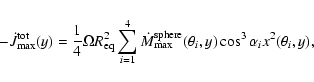 |
(6) |
Table 2:
Surface-integrated maximum mass-loss rates (expressed in
![]() yr-1) and corresponding maximum angular momentum loss
(expressed in 1037 kg m2 s
yr-1) and corresponding maximum angular momentum loss
(expressed in 1037 kg m2 s
![]()
![]() yr-1)
for the stellar models of which the equatorial parameters are listed in
Table 1, as a function of the rotation velocity. The
indication "
yr-1)
for the stellar models of which the equatorial parameters are listed in
Table 1, as a function of the rotation velocity. The
indication "![]() '' means that the star has reached the
'' means that the star has reached the
![]() -limit.
-limit.
![\begin{figure}
\par\rotatebox{270}{{\includegraphics[height=16cm,clip]{H4421.f3}}}
\end{figure}](/articles/aa/full/2004/17/aah4421/img80.gif) |
Figure 3:
|
| Open with DEXTER | |
The onset of extreme mass loss is different for the different stellar models,
occurring already at y=0.5 for stars with a high Eddington factor (above 0.6
on the entire surface, e.g. Model 3) and only at y=0.9 for stars with a very
low Eddington factor (below 0.2 everywhere on the surface such as for Models 7, 8, 9). The allowance of a possible extra force at the base of the stellar wind
thus implies that extreme mass loss might occur at critical rotation, for any
stellar model. This is in contrast to the situation where extra forces are not
taken into account and the mass loss is finite if the star is sufficiently far
from the
![]() -limit (Owocki et al. 1998; Maeder & Meynet 2000). On
the other hand, to reach the stage of extreme mass loss, one needs a rotation
rate that is at least about half the critical rate for the models we considered
here. This threshold decreases considerably for a star closer to the Eddington
limit, as we show in the next section and as was already found by Maeder &
Meynet (2000). If the extreme mass loss occurs at any lattitude, the star
can no longer be considered to be stable.
-limit (Owocki et al. 1998; Maeder & Meynet 2000). On
the other hand, to reach the stage of extreme mass loss, one needs a rotation
rate that is at least about half the critical rate for the models we considered
here. This threshold decreases considerably for a star closer to the Eddington
limit, as we show in the next section and as was already found by Maeder &
Meynet (2000). If the extreme mass loss occurs at any lattitude, the star
can no longer be considered to be stable.
In Fig. 3 we plot the ratio of
![]() and
and
![]() versus
versus
![]() as filled squares for the 9 models. The maximum mass-loss
rate increases drastically whenever the star rotates faster than half the
critical velocity. Globally, the curves behave rather similar for all 9 models
and point towards a moderate increase in
as filled squares for the 9 models. The maximum mass-loss
rate increases drastically whenever the star rotates faster than half the
critical velocity. Globally, the curves behave rather similar for all 9 models
and point towards a moderate increase in
![]() as a
function of the rotation velocity for
as a
function of the rotation velocity for
![]() and a very
steep increase for faster rotation. As expected, for models of the same
temperature, the onset of extreme mass loss occurs at higher rotation as the
luminosity decreases (compare e.g. Models 2, 4, 7).
and a very
steep increase for faster rotation. As expected, for models of the same
temperature, the onset of extreme mass loss occurs at higher rotation as the
luminosity decreases (compare e.g. Models 2, 4, 7).
The dotted line in the panels of Fig. 3 is the empirically derived relation proposed by Langer (1998) for self-regulated winds (i.e. without the inclusion of a possible extra force at the base of the wind that might increase the mass loss rate), applied to our maximum equatorial mass-loss rates for the 9 stellar models listed in Table 1. Langer (1998) neglected the oblateness of the star and the Von Zeipel effect. His relation leads to mass-loss rates that are overestimates of the true values if one does not include extra forces near the sonic point. This can be seen by comparison with the correct scaling law derived by Maeder & Meynet (2000) for a self-regulated CAK-type wind (dashed line in Fig. 3). If one allows instabilities, though, one easily ends up with larger mass-loss rates than those predicted by Langer's relation.
We find systematically a significantly higher contrast in the maximum mass-loss
rate with and without rotation than the one found by Maeder & Meynet
(2000). This finding shows that the inclusion of extra forces at the base of the
wind allows the onset of extreme mass loss at much lower rotation rates compared
to the situation where such extra forces do not occur. It is entirely
understandable that we find a larger contrast than Maeder & Meynet (2000) who
did not include any additional helpful force. Maeder & Meynet (2000) had
already derived extreme mass loss from their scaling law for stars close to the
so-called
![]() -limit. We confirm this result by direct numerical
integration of the momentum equation and we show that the onset of extreme mass
loss occurs at lower rotation rates whenever extra forces help to lift the
material at the stellar surface.
-limit. We confirm this result by direct numerical
integration of the momentum equation and we show that the onset of extreme mass
loss occurs at lower rotation rates whenever extra forces help to lift the
material at the stellar surface.
Langer (1998) computed the main sequence evolution of a 60 ![]() star with
various initial rotation rates and considered the effect of angular momentum
loss on the stellar mass-loss rate and the rotation of the star. He finds that
the coupling of mass and angular momentum loss limits the mass-loss rate of
main-sequence stars at the so-called
star with
various initial rotation rates and considered the effect of angular momentum
loss on the stellar mass-loss rate and the rotation of the star. He finds that
the coupling of mass and angular momentum loss limits the mass-loss rate of
main-sequence stars at the so-called ![]() -limit. He lists a value of
-limit. He lists a value of
![]() yr-1 which is
determined through the angular momentum loss imposed by the
yr-1 which is
determined through the angular momentum loss imposed by the ![]() -limit. We
have done quite opposite calculations as we have built up a formalism to find
the maximum mass-loss rate by line-driving from a physical model and we derived
the accompanied maximum angular momentum loss. The maximum mass loss of the
slowly rotating O-star models in our sample is indeed of the order
-limit. We
have done quite opposite calculations as we have built up a formalism to find
the maximum mass-loss rate by line-driving from a physical model and we derived
the accompanied maximum angular momentum loss. The maximum mass loss of the
slowly rotating O-star models in our sample is indeed of the order
![]() yr-1, which is compatible with Langer's (1998)
result. Hence, there seems to be general agreement between our results and
stellar evolution calculations of massive stars.
yr-1, which is compatible with Langer's (1998)
result. Hence, there seems to be general agreement between our results and
stellar evolution calculations of massive stars.
The values of the maximum mass-loss rates listed in Table 2, and
hence also those of the maximum angular momentum loss, are determined by the
adopted values of the line force parameters
![]() .
It is clear that any
future change in the values of these parameters will imply different values for
the maximum mass-loss rates. This should always be kept in mind when using them
for stellar evolution calculations. The main purpose of our work was to
investigate how high a mass can be driven in the best possible circumstances of
having a high rotation and extra forces helping to lift the wind material,
compared to the case where rotation does not occur. This ratio should not be
very sensitive to the line-force parameters. We have taken the values by
Pauldrach et al. (1986) derived from theory rather than empirical values
derived from observations. The reason why we did not rely on the empirical
values is that we needed a consistent set of
.
It is clear that any
future change in the values of these parameters will imply different values for
the maximum mass-loss rates. This should always be kept in mind when using them
for stellar evolution calculations. The main purpose of our work was to
investigate how high a mass can be driven in the best possible circumstances of
having a high rotation and extra forces helping to lift the wind material,
compared to the case where rotation does not occur. This ratio should not be
very sensitive to the line-force parameters. We have taken the values by
Pauldrach et al. (1986) derived from theory rather than empirical values
derived from observations. The reason why we did not rely on the empirical
values is that we needed a consistent set of
![]() at each temperature
at the stellar surface to be able to solve the momentum equation rather than
using a scaling law to predict the mass loss.
We also note for completeness that the empirical
at each temperature
at the stellar surface to be able to solve the momentum equation rather than
using a scaling law to predict the mass loss.
We also note for completeness that the empirical ![]() -values listed
by Lamers et al. (1995) are too low due to a small error in the code that was
used by the authors to derive them.
-values listed
by Lamers et al. (1995) are too low due to a small error in the code that was
used by the authors to derive them.
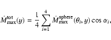
The observation that the dependence of the increase of the maximum mass-loss
rates on the ratio
![]() is quite similar over a wide range
of stellar models, as illustrated in Fig. 3, is very
fortunate. Indeed, it permits us to derive a formula that allows the prediction
of the maximum mass-loss rates for a star with a particular luminosity,
effective temperature and mass, as a function of the equatorial rotation
velocity, instead of having to calculate each time again the
is quite similar over a wide range
of stellar models, as illustrated in Fig. 3, is very
fortunate. Indeed, it permits us to derive a formula that allows the prediction
of the maximum mass-loss rates for a star with a particular luminosity,
effective temperature and mass, as a function of the equatorial rotation
velocity, instead of having to calculate each time again the
![]() -values when the stellar model parameters deviate from those
given in Table 1. With the specific goal of determining such a
statistical formulation we have performed multiple regression, using the
procedure NLMIXED of the statistical software package SAS (2002).
-values when the stellar model parameters deviate from those
given in Table 1. With the specific goal of determining such a
statistical formulation we have performed multiple regression, using the
procedure NLMIXED of the statistical software package SAS (2002).
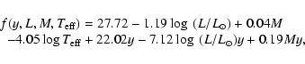
We have considered several non-linear model options and the best result was
obtained for a logistic function, which finally leads to the form
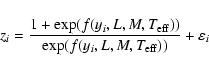
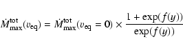
A subsequent important question is: can we find one global non-linear
model, with a good predictive power, that describes the data of the 9 models
simultaneously? If so, we can predict
![]() from the maximum mass-loss rate at zero rotation as a function of mass,
luminosity, effective temperature and equatorial rotation speed for the range of
physical parameters listed in Table 1. The coefficients for the
linear function f were hence determined from one global fit to the 81
calculated values of
from the maximum mass-loss rate at zero rotation as a function of mass,
luminosity, effective temperature and equatorial rotation speed for the range of
physical parameters listed in Table 1. The coefficients for the
linear function f were hence determined from one global fit to the 81
calculated values of
![]() (shown as full squares in
Fig. 3) simultaneously. We started from the most general
linear function for f and kept only those terms with significant coefficients.
This results in the following maximum mass-loss recipe:
(shown as full squares in
Fig. 3) simultaneously. We started from the most general
linear function for f and kept only those terms with significant coefficients.
This results in the following maximum mass-loss recipe:
As shown in Paper I (see last column in Table 3 of that paper), the maximum
mass-loss rate of a non-rotating star is between 0.5 and 1.7 times the rate of a
line-driven wind calculated with the inclusion of multiple scattering for solar
metallicity (see Vink et al. 2000). It is therefore a very good approximation
to use the values from the recipe provided by Vink et al. (2000) for solar
metallicity, in combination with our scaling law (8) and (9)
in order to find the maximum mass than can be lost by a star as a function of
rotation velocity. For completeness, we therefore repeat here the results
obtained by Vink et al. (2000):
 |
(10) |
 |
(11) |
As already emphasized by Maeder & Meynet (2000), extreme mass loss occurs for
stars near the
![]() -limit, such as luminous blue variables
(LBVs). Having included possible extra forces or
instabilities to help build up the ideal velocity gradient at the sonic point,
we can check if our models are able to explain the mass loss and the kinematical
structure of nebulae around such stars, which are indeed expected to undergo
instabilities. Weiss (2003) recently provided an overview of such structures for
several galactic and LMC LBVs. Given its extreme properties, we concentrate
mainly on the LBV
-limit, such as luminous blue variables
(LBVs). Having included possible extra forces or
instabilities to help build up the ideal velocity gradient at the sonic point,
we can check if our models are able to explain the mass loss and the kinematical
structure of nebulae around such stars, which are indeed expected to undergo
instabilities. Weiss (2003) recently provided an overview of such structures for
several galactic and LMC LBVs. Given its extreme properties, we concentrate
mainly on the LBV ![]() Carinae and we confront its observational
characteristics with our maximum mass-loss formalism.
Carinae and we confront its observational
characteristics with our maximum mass-loss formalism.
Maeder & Desjacques (2001) used their mass-loss scaling law to derive mass flux
plots of stars like ![]() Carinae in the two cases of a shell ejection and of
a constant wind. A much more systematic study of the shaping of LBV nebulae in
terms of radiatively driven winds was provided by Dwarkadas & Owocki
(2002). They obtained an equatorial mass-loss rate that is about 1/5 of its
polar value. They also provided density contours derived from wind simulations
for which they fixed the maximum mass-loss rate to
Carinae in the two cases of a shell ejection and of
a constant wind. A much more systematic study of the shaping of LBV nebulae in
terms of radiatively driven winds was provided by Dwarkadas & Owocki
(2002). They obtained an equatorial mass-loss rate that is about 1/5 of its
polar value. They also provided density contours derived from wind simulations
for which they fixed the maximum mass-loss rate to
![]() yr-1and the maximum polar wind velocity to 2000 km s-1. Their simulations
showed convincingly that radiatively driven wind theory leads in a natural way
to a latitudinal dependence in velocity and mass loss for rotating stars, with
both a higher mass flux and a higher terminal velocity from the pole than from
the equator (in the absence of a bi-stability jump). They also provided a model
for
yr-1and the maximum polar wind velocity to 2000 km s-1. Their simulations
showed convincingly that radiatively driven wind theory leads in a natural way
to a latitudinal dependence in velocity and mass loss for rotating stars, with
both a higher mass flux and a higher terminal velocity from the pole than from
the equator (in the absence of a bi-stability jump). They also provided a model
for ![]() Carinae in which they assumed a pre-outburst wind with a polar
velocity of 700 km s-1 and a mass loss of
Carinae in which they assumed a pre-outburst wind with a polar
velocity of 700 km s-1 and a mass loss of
![]() yr-1,
and an outburst period of 20 years during which the velocity was assumed not to
change but during which the mass loss increased to
yr-1,
and an outburst period of 20 years during which the velocity was assumed not to
change but during which the mass loss increased to
![]() yr-1. The density contour plots they obtained in this way
indeed resemble
yr-1. The density contour plots they obtained in this way
indeed resemble ![]() Carinae's Homunculus Nebula.
Carinae's Homunculus Nebula.
Recent progress in determining the observational properties of ![]() Carinae
is impressive. Hillier et al. (2001) have derived observational properties of
the star from HST/STIS spectra and require a current mass-loss rate of
Carinae
is impressive. Hillier et al. (2001) have derived observational properties of
the star from HST/STIS spectra and require a current mass-loss rate of
![]() yr-1 to obtain a good fit to the spectrum. More
recently, van Boekel et al. (2003) have obtained a direct measurement of the
size and the shape of the stellar wind of
yr-1 to obtain a good fit to the spectrum. More
recently, van Boekel et al. (2003) have obtained a direct measurement of the
size and the shape of the stellar wind of ![]() Carinae from interferometric
data gathered with the VLTI. They derive an even higher current mass-loss rate
of
Carinae from interferometric
data gathered with the VLTI. They derive an even higher current mass-loss rate
of
![]() yr-1, assuming a spherically
symmetric clumped wind. Smith et al. (2003) found the wind structure of the
star to be axisymmetric and variable in time, with higher velocities (of order
600-1 000 km s-1) and higher densities at the pole than at the
equator from new STIS spectra.
yr-1, assuming a spherically
symmetric clumped wind. Smith et al. (2003) found the wind structure of the
star to be axisymmetric and variable in time, with higher velocities (of order
600-1 000 km s-1) and higher densities at the pole than at the
equator from new STIS spectra.
An important question is whether the high observed mass-loss rate of
![]() Carinae can be explained in terms of radiatively driven wind theory.
Our formalism is ideally suited to answer this question as it allows for the
influence of instabilities at the base of the wind. We have therefore solved the
momentum equation for stellar parameters appropriate for
Carinae can be explained in terms of radiatively driven wind theory.
Our formalism is ideally suited to answer this question as it allows for the
influence of instabilities at the base of the wind. We have therefore solved the
momentum equation for stellar parameters appropriate for ![]() Carinae and
determined the maximum mass-loss rates as explained in Sect. 3 for models that
have not yet reached the
Carinae and
determined the maximum mass-loss rates as explained in Sect. 3 for models that
have not yet reached the
![]() -limit but are only barely below this
limit. We have kept a large degree of freedom on stellar parameters in the first
instance as these are not well known for
-limit but are only barely below this
limit. We have kept a large degree of freedom on stellar parameters in the first
instance as these are not well known for ![]() Carinae.
Carinae.
It is not our intention to provide a fully explored set of models that lead to
the observed mass loss. Rather we emphasize that such models indeed were found
by us. One such model has the following characteristics:
![]() ,
,
![]() ,
,
![]() ,
,
![]() K,
K,
![]() K,
K,
![]() ,
,
![]() ,
,
![]() km s-1,
km s-1,
![]() ,
,
![]() .
The
highest possible mass-loss rates we obtained from integration of the momentum
equation are in this case
.
The
highest possible mass-loss rates we obtained from integration of the momentum
equation are in this case
![]() yr-1 at the pole
and
yr-1 at the pole
and
![]() yr-1 at the equator, leading to a
surface-integrated mass loss of
yr-1 at the equator, leading to a
surface-integrated mass loss of
![]() yr-1. The mass-loss
contrast of a factor three between the pole and the equator (with a higher mass
loss rate from the pole), together with the factor 0.5 for the maximum velocity,
(with a higher outflow velocity from the equator - see below) leads to a
density contrast of a factor 6. This is compatible with the factor 5 found
by Dwarkadas & Owocki (2002), although they obtain a higher velocity at the
pole than at the equator. We stress that the listed model parameters are just
one set that lead to the appropriate mass-loss rate and there may be several
others that do so as well. We also stress that much more extreme mass-loss
rates are easily reached for stars above the
yr-1. The mass-loss
contrast of a factor three between the pole and the equator (with a higher mass
loss rate from the pole), together with the factor 0.5 for the maximum velocity,
(with a higher outflow velocity from the equator - see below) leads to a
density contrast of a factor 6. This is compatible with the factor 5 found
by Dwarkadas & Owocki (2002), although they obtain a higher velocity at the
pole than at the equator. We stress that the listed model parameters are just
one set that lead to the appropriate mass-loss rate and there may be several
others that do so as well. We also stress that much more extreme mass-loss
rates are easily reached for stars above the
![]() -limit (i.e. with
-limit (i.e. with
![]() ,
as shown in Fig. 3 and listed
in Table 2 in Sect. 3. However, the purpose of our investigation of
,
as shown in Fig. 3 and listed
in Table 2 in Sect. 3. However, the purpose of our investigation of
![]() Carinae was to search for models with a "natural'' line-driven outflow
based on an ideal velocity gradient at the sonic point that explains the
observed mass loss rather than having to invoke a specific outburst with a much
increased ad-hoc mass-loss rate as often assumed in the literature. From the
point of view of the high mass loss we have succeeded in finding such models.
Carinae was to search for models with a "natural'' line-driven outflow
based on an ideal velocity gradient at the sonic point that explains the
observed mass loss rather than having to invoke a specific outburst with a much
increased ad-hoc mass-loss rate as often assumed in the literature. From the
point of view of the high mass loss we have succeeded in finding such models.
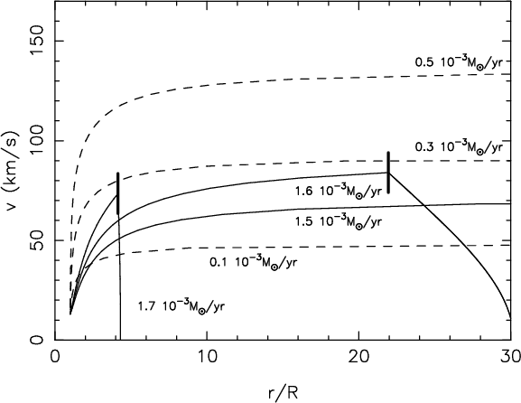 |
Figure 4:
Some velocity laws resulting from integration of the momentum
equation for stellar parameters appropriate for |
| Open with DEXTER | |
While large uncertainties of several hundred km s-1 exist for the terminal
wind velocity of ![]() Carinae we could not find a model below the
Carinae we could not find a model below the
![]() -limit that explains both the observed mass-loss rate and the wind
velocity of the star in full details. For appropriate mass-loss rates, we always
end up with a much lower wind velocity, similar to the one shown in
Fig. 4. Note that Maeder & Desjaques (2001) and Dwarkadas & Owocki
(2002) assumed values for the wind speeds and mass-loss rates to end up
with an acceptable configuration from scaling laws. We provide a fully
consistent estimate of the wind velocity and maximum mass loss. The velocities
we derive in such a way for stars close to the
-limit that explains both the observed mass-loss rate and the wind
velocity of the star in full details. For appropriate mass-loss rates, we always
end up with a much lower wind velocity, similar to the one shown in
Fig. 4. Note that Maeder & Desjaques (2001) and Dwarkadas & Owocki
(2002) assumed values for the wind speeds and mass-loss rates to end up
with an acceptable configuration from scaling laws. We provide a fully
consistent estimate of the wind velocity and maximum mass loss. The velocities
we derive in such a way for stars close to the
![]() -limit are in
general in very good agreement with the expansion velocities observed by Weis
(2003) for several LBVs, except for
-limit are in
general in very good agreement with the expansion velocities observed by Weis
(2003) for several LBVs, except for ![]() Carinae for which they are an order
of magnitude too low.
Carinae for which they are an order
of magnitude too low.
Given the observed geometry of the Homunculus of ![]() Carinae, the wind
velocity near the equator must be significantly lower than at the pole. In our
model shown in Fig. 4 this would correspond to the velocity curve
obtained for
Carinae, the wind
velocity near the equator must be significantly lower than at the pole. In our
model shown in Fig. 4 this would correspond to the velocity curve
obtained for
![]() yr-1 at the equator. It is quite
easy to imagine that the equatorial region would undergo a different effect on
its local mass loss from an instability than the pole. A non-radial axisymmetric
even oscillation mode, for instance, is just one simple example of an
instability that could lead to such an effect. It is clear that our formalism
has the potential to lead to very different geometries of the density
distribution around a rotating star because we have left the cause of obtaining
the ideal velocity gradient at the sonic point unspecified. Several natural
large-amplitude phenomena occur at the surface of massive stars (such as stellar
oscillations or a complex magnetic field) and may indeed help in the onset of
the local mass loss.
yr-1 at the equator. It is quite
easy to imagine that the equatorial region would undergo a different effect on
its local mass loss from an instability than the pole. A non-radial axisymmetric
even oscillation mode, for instance, is just one simple example of an
instability that could lead to such an effect. It is clear that our formalism
has the potential to lead to very different geometries of the density
distribution around a rotating star because we have left the cause of obtaining
the ideal velocity gradient at the sonic point unspecified. Several natural
large-amplitude phenomena occur at the surface of massive stars (such as stellar
oscillations or a complex magnetic field) and may indeed help in the onset of
the local mass loss.
We conclude that we have found radiatively-driven wind models below the
![]() -limit that explain in a natural way the huge currently observed
mass-loss rate of
-limit that explain in a natural way the huge currently observed
mass-loss rate of ![]() Carinae and its spatial distribution. From the point
of view of mass loss we would therefore not need any different physical
mechanism or a specific eruption to explain the star's nebula and geometry. Our
models, however, have too low a wind velocity. We do point out that all
other LBVs have expansion velocities that are entirely compatible with the
predicted maximum wind velocities of our models.
Carinae and its spatial distribution. From the point
of view of mass loss we would therefore not need any different physical
mechanism or a specific eruption to explain the star's nebula and geometry. Our
models, however, have too low a wind velocity. We do point out that all
other LBVs have expansion velocities that are entirely compatible with the
predicted maximum wind velocities of our models.
We determined the maximum mass-loss rates of stars by means of a wind that is lifted out of the potential well by radiation pressure on spectral lines, taking into account rotation. Our calculations were done for a simplistic CAK-type description of the line driving, including the oblateness of the star and the Von Zeipel effect and allowing for the possible presence of an extra force or an unspecified instability at the base of the wind (at or below the sonic point) that might increase the mass-loss rate. The maximum mass-loss rates were determined explicitly for 9 stellar models, which are representative for massive stars at different evolutionary stages and not too close to the Eddington limit. All rotating models have higher mass-loss rates at the pole than at the equator, the contrast increasing as the rotation increases. This is in agreement with previous studies of self-regulated winds in the absence of a rotationally induced bi-stability jump (Pelupessy et al. 2000), as shown by Dwarkadas & Owocki (2002). For moderately to rapidly rotating stars we find maximum mass-loss rates that are significantly higher than those of non-rotating stars. In particular, all OB stars with near-critical rotation can have extreme mass loss in the presence of surface instabilities. From comparison of our results with those by Maeder & Meynet (2000) we conclude that the onset of extreme mass loss occurs at lower rotation rates when allowing an instability to help increase the mass-loss rate or lift the material at the base of the wind.
We provide the maximum loss of angular momentum as function of the stellar parameters and of the rotational velocity for all considered models. It would be worthwhile to compare these angular momentum losses with those used in stellar evolution codes.
We provide a formula to predict the maximum mass-loss rate for
stars with a luminosity not too different from
![]() .
It
was derived from multiple regression using the results of our detailed numerical
integration of the momentum equation for 9 models. This formula can easily be
combined with mass-loss estimates based on multiple scattering for non-rotating
stars (Vink et al. 2000, 2001). The use of the formula provided by Maeder &
Meynet (2000) allows one to find the mass lost by massive stars in the presence
of rotation without the occurrence of instabilities while our formula leads to
the maximum amount of mass that can be lost due to a line-driven wind in a
rotating star that undergoes unspecified instabilities which help to reach the
optimum velocity gradient at the sonic point.
.
It
was derived from multiple regression using the results of our detailed numerical
integration of the momentum equation for 9 models. This formula can easily be
combined with mass-loss estimates based on multiple scattering for non-rotating
stars (Vink et al. 2000, 2001). The use of the formula provided by Maeder &
Meynet (2000) allows one to find the mass lost by massive stars in the presence
of rotation without the occurrence of instabilities while our formula leads to
the maximum amount of mass that can be lost due to a line-driven wind in a
rotating star that undergoes unspecified instabilities which help to reach the
optimum velocity gradient at the sonic point.
By means of integration of the momentum equation for the specific case of the
LBV ![]() Carinae we have found models below the
Carinae we have found models below the
![]() -limit that
lead to realistic predictions of the huge mass loss observed for this star and
of its latitudinal distribution. In general, we are able to explain the
combination of high mass loss and low wind velocities observed in LBVs. We were
unable, however, to find a model below the
-limit that
lead to realistic predictions of the huge mass loss observed for this star and
of its latitudinal distribution. In general, we are able to explain the
combination of high mass loss and low wind velocities observed in LBVs. We were
unable, however, to find a model below the
![]() -limit that predicts
the high mass-loss rate in combination with the measured high wind velocity of
-limit that predicts
the high mass-loss rate in combination with the measured high wind velocity of
![]() Carinae itself.
Carinae itself.
Acknowledgements
The authors are much indebted to prof. André Maeder for his constructive criticism on an earlier draft of the paper, which helped them to make significant improvements to the study. C.A. is grateful to profs. Stan Owocki, Joachim Puls, Rens Waters and drs. Roy van Boekel and Rich Townsend for stimulating discussions.