We can think of a lensed quasar as taking the Hubble time, shrinking it by
A&A 414, 425-428 (2004)
DOI: 10.1051/0004-6361:20034184
P. Saha
Astronomy Unit,
Queen Mary and Westfield College,
University of London,
London E1 4NS, UK
Observatoire astronomique,
11 rue de l'Université,
67000 Strasbourg, France
Received 12 August 2003 / Accepted 18 September 2003
Abstract
We can think of a lensed quasar as taking the Hubble time,
shrinking it by ![]() 10-11, and then presenting the result to us
as a time delay; the shrinking factor is of the order of fractional
sky-area that the lens occupies. This cute fact is a straightforward
consequence of lensing theory, and enables a simple rescaling of time
delays. Observed time delays have a 40-fold range, but after
rescaling the range reduces to 5-fold. The latter range depends on
details of the lens and lensing configuration - for example, quads
have systematically shorter rescaled time delays than doubles - and is
as expected from a simple model. The hypothesis that observed
time-delay lenses all come from a generalized-isothermal family can be
ruled out. But there is no indication of drastically different
populations either.
10-11, and then presenting the result to us
as a time delay; the shrinking factor is of the order of fractional
sky-area that the lens occupies. This cute fact is a straightforward
consequence of lensing theory, and enables a simple rescaling of time
delays. Observed time delays have a 40-fold range, but after
rescaling the range reduces to 5-fold. The latter range depends on
details of the lens and lensing configuration - for example, quads
have systematically shorter rescaled time delays than doubles - and is
as expected from a simple model. The hypothesis that observed
time-delay lenses all come from a generalized-isothermal family can be
ruled out. But there is no indication of drastically different
populations either.
Key words: Gravitational lensing - galaxies: quasars: general
Most of the observables in gravitational lensing (image positions and
magnifications) are intrinsically dimensionless. The exception is the
time delay between images, which takes its dimensionality straight
from the universe![]() :
:
![]() .
This remarkable fact is
the essential reason for much research effort going into measuring
time delays. The observations have been increasingly successful - in
1995 there was but one controversial time delay, currently there are
nine non-controversial ones. These are summarized in Table 1
below.
.
This remarkable fact is
the essential reason for much research effort going into measuring
time delays. The observations have been increasingly successful - in
1995 there was but one controversial time delay, currently there are
nine non-controversial ones. These are summarized in Table 1
below.
But curiously, even as the image and time delay data have improved,
the error bars on the inferred H0 have not. As an example,
consider 0957+561. Between Kundic et al. (1997) and Oscoz et al. (2001) the
time-delay value changed by only 2%. But meanwhile, whereas
Kundic et al. (1997) quote
![]() (95% confidence) in the usual
units of
(95% confidence) in the usual
units of
![]() ,
Bernstein & Fischer (1999) with more
imaging and more modelling conclude that the data imply only
77+29-24, while Keeton et al. (2000) assert that further data on
the lensed host galaxy invalidates all previously published models,
and they decline to give an H0 estimate at all. Basically, the
problem is that simple lens models are unable to fit the images to the
mas-level demanded by current data, while more complicated models can
fit the data but are non-unique and can produce identical observables
from very different values of H0.
,
Bernstein & Fischer (1999) with more
imaging and more modelling conclude that the data imply only
77+29-24, while Keeton et al. (2000) assert that further data on
the lensed host galaxy invalidates all previously published models,
and they decline to give an H0 estimate at all. Basically, the
problem is that simple lens models are unable to fit the images to the
mas-level demanded by current data, while more complicated models can
fit the data but are non-unique and can produce identical observables
from very different values of H0.
Modellers have responded to this dilemma with two strategies. One is to try to identify simple models that both have enough parameters to fit or nearly fit the data and can be justified on galactic-structure grounds; Kochanek (2003) is typical of these. The other strategy is to try to explore the space of all plausible models allowed by the data; Raychaudhury et al. (2003) is a recent example. For a review by authors representing different points of view see Courbin et al. (2003).
In the current context of good data and active modelling but no
consensus on models, it is interesting to step back and pose some
questions that tend to get obscured in the details of modelling.
First, we can think of the purpose of modelling time-delay lenses as
being to discover one dimensionless number, the factor relating
![]() and H0-1. What contributions to this number are
well-constrained and what are poorly constrained? What range of
values do the data imply for the poorly-constrained part? Is that
range systematically different for doubles and quads, and/or for
isolated lensing galaxies versus interacting galaxies? And is that
range consistent with what we expect from popular models? Nine
systems is a small sample, but it is enough to provide preliminary
answers to these questions, and to do so is the aim of this paper.
and H0-1. What contributions to this number are
well-constrained and what are poorly constrained? What range of
values do the data imply for the poorly-constrained part? Is that
range systematically different for doubles and quads, and/or for
isolated lensing galaxies versus interacting galaxies? And is that
range consistent with what we expect from popular models? Nine
systems is a small sample, but it is enough to provide preliminary
answers to these questions, and to do so is the aim of this paper.
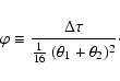
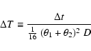
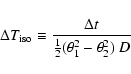
In lensing theory the arrival time can be written as
![\begin{displaymath}t({\setbox 0\hbox to 0pt{\hss$\scriptstyle\rightarrow$ } \the...
...htarrow$ } \theta\kern.6ex\raise 1.6ex\box0\kern-.2ex})\right]
\end{displaymath}](/articles/aa/full/2004/05/aa0184/img10.gif) |
(1) |
 |
(3) |
 |
(6) |
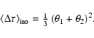
For isothermal lenses, ![]() ranges from 0 to 8, averaging
ranges from 0 to 8, averaging
![]() .
To see this, recall that for isothermals,
.
To see this, recall that for isothermals,
![]() and note that
and note that ![]() could be anywhere in
the Einstein ring. Hence
could be anywhere in
the Einstein ring. Hence
![]() and using (7)
gives
and using (7)
gives
Witt et al. (2000, hereafter WMK) show that
![]() is not
restricted to isothermals but is valid for a large family of
generalized-isothermal lenses, and argue that it will be generally
applicable in nature. If so,
is not
restricted to isothermals but is valid for a large family of
generalized-isothermal lenses, and argue that it will be generally
applicable in nature. If so, ![]() could be eliminated
altogether. We can readily test if this is the case.
could be eliminated
altogether. We can readily test if this is the case.
We now present the obvious comparison of the scaled time delays
![]() with current data.
with current data.
Table 1 lists the relevant quantities for the various
time-delay systems. The time delays references are given in the
table, and the other data are taken from the CASTLES survey and
compilation by Kochanek et al. (1998). For quads, only the first and last
images (that is, the longest time delay) are considered, to enable a
simple comparison with doubles. There are some caveats to the values
of ![]() and
and ![]() :
for 1830 and 0218 the lens-centre is
very uncertain and hence
:
for 1830 and 0218 the lens-centre is
very uncertain and hence
![]() are especially uncertain,
for 1608 the lens is apparently an interacting pair of galaxies, and
0957 and 0911 are in clusters and hence have large
lensing contributions from other galaxies.
are especially uncertain,
for 1608 the lens is apparently an interacting pair of galaxies, and
0957 and 0911 are in clusters and hence have large
lensing contributions from other galaxies.
Table 1: Summary of time-delay data.
Figure 1 shows ![]() against
against ![]() for the
currently known time-delay systems. Since error bars on time delays
are typically a few percent they are not shown here. We notice three
things:
for the
currently known time-delay systems. Since error bars on time delays
are typically a few percent they are not shown here. We notice three
things:
![\begin{figure}
\includegraphics[width=8cm,clip]{saha_fig1.eps}
\end{figure}](/articles/aa/full/2004/05/aa0184/img50.gif) |
Figure 1:
Plot of the scaled time delay |
| Open with DEXTER | |
![\begin{figure}
\par\includegraphics[width=8cm,clip]{saha_fig2.eps}
\end{figure}](/articles/aa/full/2004/05/aa0184/img51.gif) |
Figure 2: As in Fig. 1, but omitting the D factor in the scaled time delay. |
| Open with DEXTER | |
We can also compare
![]() against the data to test
whether the lenses belong to the generalized isothermal family studied
by WMK. Figure
3 shows
against the data to test
whether the lenses belong to the generalized isothermal family studied
by WMK. Figure
3 shows
![]() against
against ![]() for the same
systems. We notice the following
for the same
systems. We notice the following
Whereas
![]() is rejected, are other scalings possible that
improve upon
is rejected, are other scalings possible that
improve upon ![]() ? L.L.R. Williams (personal communication)
points out that the definition (Eq. 5) of
? L.L.R. Williams (personal communication)
points out that the definition (Eq. 5) of ![]() considers the size of the lens but not its asymmetry, and that if we
multiply
considers the size of the lens but not its asymmetry, and that if we
multiply
![]() in the definition by a further factor
of
in the definition by a further factor
of
![]() as a measure of
asymmetry, then the scaled time delays would range over a factor of
only 2.5, with no significant trend. But the meaning of such an
asymmetry correction in terms of lensing theory is not known.
as a measure of
asymmetry, then the scaled time delays would range over a factor of
only 2.5, with no significant trend. But the meaning of such an
asymmetry correction in terms of lensing theory is not known.
![\begin{figure}
\par\includegraphics[width=8cm,clip]{saha_fig3.eps}
\end{figure}](/articles/aa/full/2004/05/aa0184/img55.gif) |
Figure 3:
|
| Open with DEXTER | |
From the above, it appears that the scatter in ![]() reflects a
range of mass profiles and source positions, and that its value must
be inferred for each lens by detailed modelling. But without going
into detailed models for nine lenses, we can at least check whether
the observed range of
reflects a
range of mass profiles and source positions, and that its value must
be inferred for each lens by detailed modelling. But without going
into detailed models for nine lenses, we can at least check whether
the observed range of ![]() is plausible.
is plausible.
Figure 4 shows such a check. The main plot is of ![]() against the area
against the area
![]() for an example model (an
elliptical isothermal potential plus external shear.) The value of
for an example model (an
elliptical isothermal potential plus external shear.) The value of
![]() is shown for different source positions, the two loops
corresponding to source positions along the two caustics (actually
just inside the caustics, to avoid computational problems). Quads are
below the lower loop, with
is shown for different source positions, the two loops
corresponding to source positions along the two caustics (actually
just inside the caustics, to avoid computational problems). Quads are
below the lower loop, with
![]() .
Doubles are between the
two loops, with
.
Doubles are between the
two loops, with
![]()
![]() . The values
are model-dependent - for example, a steeper model will have both
loops somewhat higher. Also, the value of
. The values
are model-dependent - for example, a steeper model will have both
loops somewhat higher. Also, the value of
![]() depends on the source position: smaller for sources along the long
axis of the potential, larger for sources perpendicular to that axis.
But with these qualifications, Figure 4 shows that the
general ranges of
depends on the source position: smaller for sources along the long
axis of the potential, larger for sources perpendicular to that axis.
But with these qualifications, Figure 4 shows that the
general ranges of ![]() ,
including the separation of quads and
doubles, is just as it is in the data, and there is no evidence that
the observed systems come from drastically different populations of
lenses.
,
including the separation of quads and
doubles, is just as it is in the data, and there is no evidence that
the observed systems come from drastically different populations of
lenses.
![\begin{figure}
\par\includegraphics[width=3.6cm,clip]{saha_fig4a.eps}\hspace*{2m...
...\includegraphics[width=7.2cm,clip]{saha_fig4c.eps}\hspace*{0.5mm}}\end{figure}](/articles/aa/full/2004/05/aa0184/img58.gif) |
Figure 4:
Computation of |
| Open with DEXTER | |
We see in this paper a new interpretation of lensing time delays:
![]() is H0-1 shrunk by the lens's covering factor on the
sky, times a number of the order of unity. On separating off a redshift
dependent-term (also of order unity) we are left with a number
is H0-1 shrunk by the lens's covering factor on the
sky, times a number of the order of unity. On separating off a redshift
dependent-term (also of order unity) we are left with a number ![]() (say) that summarizes the dependence on details of the lens
and lens configuration.
(say) that summarizes the dependence on details of the lens
and lens configuration.
Using these ideas, we can rescale the observed time delays for the
nine currently-measured systems. The observed time delays range over
a factor of 40, but the rescaled delays range over a factor of 5. The
latter is the inferred range of ![]() ,
and moreover it appears
that
,
and moreover it appears
that
![]() for quads and
for quads and
![]() .
Reassuringly, the same spread in
.
Reassuringly, the same spread in ![]() is reproduced by a simple
model.
is reproduced by a simple
model.
Using rescaled time-delays we can also test the hypothesis that the observed lenses all belong to a generalized-isothermal family. This hypothesis is ruled out: it over-predicts time delaysfor large lenses. On the other hand, there is no indication that the known time-delay systems come from drastically different types of lenses.
In Figs. 1 to 3 we have some points
(xi,yi) and we want to know whether there is any trend in the
scatter. There are many statistical tests relating to the
significance of trends in data, but none of the standard ones address
quite this question. However, it is not difficult to design a
suitable statistical test. Let us pose the question: what is the
probability of improving the fit to
![]() by shuffling the
yi? If nearly all shufflings reduce the
by shuffling the
yi? If nearly all shufflings reduce the
![]() we would
conclude that the data have a trend.
we would
conclude that the data have a trend.
In the familiar straight-line fit, the slope is monotonic in
![]() .
Hence as a statistic,
.
Hence as a statistic,
![]() is equivalent to
the slope.
is equivalent to
the slope.
In the main text, I use the phrase "significant at the 95% level''
to mean that 5% of shufflings increase the
![]() .
Statisticians might use a phrase like "p-value of 95%''.
.
Statisticians might use a phrase like "p-value of 95%''.
Acknowledgements
I am grateful to Rodrigo Ibata and Liliya Williams, who contributed some fruitful suggestions.