A&A 411, 543-552 (2003)
DOI: 10.1051/0004-6361:20031491
Stellar evolution with rotation and magnetic fields
I. The relative importance of rotational and magnetic effects
A. Maeder - G. Meynet
Geneva Observatory 1290 Sauverny, Switzerland
Received 28 May 2003 / Accepted 15 September 2003
Abstract
We compare the current effects of rotation in stellar evolution to those of
the magnetic field created by the Tayler instability. In stellar
regions, where a magnetic field can be generated by the dynamo due to differential
rotation (Spruit 2002), we find that the growth rate
of the magnetic instability is much faster
than for the thermal instability. Thus, meridional circulation is small
with
respect to the magnetic fields, both for the transport of
angular momentum and of chemical elements. Also, the horizontal coupling by
the magnetic field, which reaches values of a few 105 G, is much more important than the effects
of the horizontal turbulence. The field, however, is not sufficient to distort the shape
of the equipotentials. We impose the condition that the energy of the magnetic field
created by the Tayler-Spruit
dynamo cannot be larger than the energy excess present in the differential
rotation. This leads to a criterion for the existence of the magnetic field
in stellar interiors.
Numerical tests are made in a rotating star model of
 rotating with
an initial velocity of 300 km s-1. We find that the coefficients of diffusion for the transport
of angular momentum by the magnetic field are several orders of magnitude
larger than the transport coefficients for meridional circulation and shear mixing.
The same applies to the diffusion coefficients for the chemical elements; however,
very close to the core, the strong
rotating with
an initial velocity of 300 km s-1. We find that the coefficients of diffusion for the transport
of angular momentum by the magnetic field are several orders of magnitude
larger than the transport coefficients for meridional circulation and shear mixing.
The same applies to the diffusion coefficients for the chemical elements; however,
very close to the core, the strong  -gradient reduces the mixing by the magnetic instability
to values not too different from the case without magnetic field. We also find that magnetic instability
is present throughout the radiative envelope, with the exception of the very outer
layers, where differential rotation is insufficient to build the field, a fact consistent
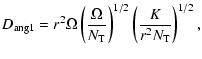
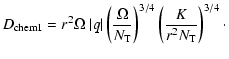
with the lack of evidence of strong fields at the surface of massive stars.
However, the equilibrium situation reached by a rotating star with magnetic field
and rotation is still to be ascertained.
-gradient reduces the mixing by the magnetic instability
to values not too different from the case without magnetic field. We also find that magnetic instability
is present throughout the radiative envelope, with the exception of the very outer
layers, where differential rotation is insufficient to build the field, a fact consistent
with the lack of evidence of strong fields at the surface of massive stars.
However, the equilibrium situation reached by a rotating star with magnetic field
and rotation is still to be ascertained.
Key words: stars: rotation - stars: magnetic field - stars: evolution
The inclusion of new physical effects in stellar evolution greatly improves the
comparisons with observations. About twenty years ago the impact of mass loss
by stellar winds on the evolution was found to be large. However, some significant discrepancies
remained and the inclusion of rotation has enabled substantial progress
in the comparisons with observed chemical abundances, with number counts and
with chemical evolution of galaxies (cf. Langer et al. 1999;
Maeder & Meynet 2000).
The magnetic field is the next, but certainly
not the last, in this series of effects which may influence all the
outputs of stellar evolution.
In this work, we focus mainly on the relative importance of the effects
of the magnetic field and of rotational instabilities to try to determine which effects can be let aside
and what must be considered a priority. Section 2 summarizes the main effects of the
magnetic field we are considering here following Spruit (1999, 2002).
Section 3 compares
the characteristic times of meridional circulation and of magnetic field
instabilities. Section 4 considers what happens to the horizontal turbulence
in presence of magnetic fields. Section 5 shows a new physical limit on the occurrence
of the magnetic field
in rotating stars. Section 6 gives some numerical values on the size of magnetic and
rotational effects in the
case of a
star. Section 7 presents the conclusions.
Let us collect here some basic expressions and concepts we need below.
Spruit (1999, 2002) has shown that the magnetic field
can be created in radiative layers of stars in differential rotation.
Even a small toroidal field is subject to an instability (called Tayler instability
by Spruit), which creates a vertical field component. Differential rotation winds up
this vertical component, so that many new horizontal field lines are produced. These
horizontal field lines become progressively closer and denser
in a star in a state of differential rotation, and therefore
a much stronger horizontal field is built. This is the dynamo processs described by Spruit.
The Tayler instability is a pinch-type instability. As shown by
Spruit (1999), it has a very low threshold and is characterized by a short
timescale. Also it is the first instability to occur. The magnetic shear instability
may be present, but it is of much less importance (Spruit 1999).
The instability occurs in radiative zones and two cases are
considered by Spruit (1999,
2002) depending on the thermal and -gradients
through the associated oscillation frequencies,
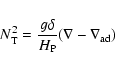 |
(1) |
and
 |
(2) |
The thermodynamic coefficients  and
and  are defined as follows
 and
and
 .
The quantity
.
The quantity  is the local pressure scale height.
Following Spruit, we call case 0 the case where the -gradient dominates
over the thermal gradient, i.e. when
is the local pressure scale height.
Following Spruit, we call case 0 the case where the -gradient dominates
over the thermal gradient, i.e. when
 .
Case 1 applies when the thermal gradient is the main restoring force, i.e.
when
.
Case 1 applies when the thermal gradient is the main restoring force, i.e.
when
 .
Let us point out that cases 0 and 1 are the two simpler limits of a more general
case, where a proper account of both thermal and
effects would be made.
We may wonder whether we miss some important physical situations with this
simplification. Indeed, numerical tests show that in practice the intermediate
situation between cases 0 and 1 introduced by Spruit concerns a small but
significant part of the star as shown in Fig. 2.
In this part, cases 0 and 1 give diffusion coefficients which have
the same order of magnitude, therefore the general effect is correctly described.
However, there is little doubt that in future
the general non-adiabatic case has to be examined in detail.
.
Let us point out that cases 0 and 1 are the two simpler limits of a more general
case, where a proper account of both thermal and
effects would be made.
We may wonder whether we miss some important physical situations with this
simplification. Indeed, numerical tests show that in practice the intermediate
situation between cases 0 and 1 introduced by Spruit concerns a small but
significant part of the star as shown in Fig. 2.
In this part, cases 0 and 1 give diffusion coefficients which have
the same order of magnitude, therefore the general effect is correctly described.
However, there is little doubt that in future
the general non-adiabatic case has to be examined in detail.
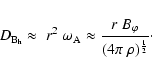
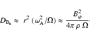
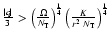
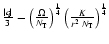
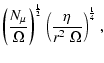
The growth rate of the magnetic instability is
 |
(3) |
where
 is the Alfven frequency, i.e. the frequency
of magnetic waves. As shown by Pitts & Tayler (1986), the
reduction factor
is the Alfven frequency, i.e. the frequency
of magnetic waves. As shown by Pitts & Tayler (1986), the
reduction factor
 in
Eq. (3) results from the Coriolis
force in a star rotating with angular velocity
in
Eq. (3) results from the Coriolis
force in a star rotating with angular velocity  .
The Alfvén frequency is
.
The Alfvén frequency is
 |
(4) |
The magnetic instability works only if the unstable displacements do
not lose too much energy against the stable stratification. For this
to be the case, the radial displacements (against the buoyancy force)
must be small compared to the horizontal displacements. Taking ras a maximum for the horizontal displacements, this sets an upper
limit on the radial length scale
lr0, 1 of the displacements,
 |
(5) |
and
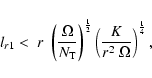 |
(6) |
where the indices 0 or 1 refer to the two cases considered. The term
K is the thermal diffusivity
 ,
where the other
quantities have their usual meaning in stellar structure.
There is also a minimal extent of the magnetic instability,
below which it is quickly dissipated by magnetic diffusivity,
,
where the other
quantities have their usual meaning in stellar structure.
There is also a minimal extent of the magnetic instability,
below which it is quickly dissipated by magnetic diffusivity,
 |
(7) |
where  is the diffusivity of the magnetic field.
The combination of Eq. (7) with Eqs. (5) and (6) leads
to a minimum value of the Alfvén frequency for the occurrence of the magnetic
instability in the two cases considered,
is the diffusivity of the magnetic field.
The combination of Eq. (7) with Eqs. (5) and (6) leads
to a minimum value of the Alfvén frequency for the occurrence of the magnetic
instability in the two cases considered,
These are the conditions in order that the magnetic field overcomes the
restoring force of buoyancy. In addition in the second case, the effects of the
thermal diffusivity described by K are also accounted for. The corresponding
maximum radial dimensions of the instabilities are given by the above
Eqs. (5) and (6).
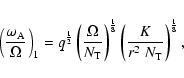
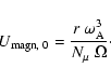
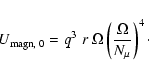
Spruit (2002; Eqs. (18) and (19))
considers the amplification timescale necessary to double the component
 starting from the radial component
  over the largest
characteristic lengths defined by Eqs. (5) and (6). He assumes the equality
of the amplification timescale
with the timescale for the damping by magnetic diffusivity over the above
lenghtscales. In this way, he obtains
the expressions for the
Alfvén frequency. In the first case, where
over the largest
characteristic lengths defined by Eqs. (5) and (6). He assumes the equality
of the amplification timescale
with the timescale for the damping by magnetic diffusivity over the above
lenghtscales. In this way, he obtains
the expressions for the
Alfvén frequency. In the first case, where  dominates, this is
 |
(10) |
where
 .
Thus, we
see that the Alfvén frequency (a measure of the field amplitude)
depends on the differential rotation parameter and on the ratio
of the angular velocity to the Brunt-Vaisala frequency.
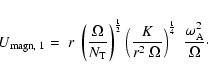
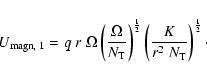
When thermal diffusion is accounted for (
negligible), one has
.
Thus, we
see that the Alfvén frequency (a measure of the field amplitude)
depends on the differential rotation parameter and on the ratio
of the angular velocity to the Brunt-Vaisala frequency.
When thermal diffusion is accounted for (
negligible), one has
 |
(11) |
there the thermal diffusivity also intervenes. A few other recalls will be made when
necessary.
Table 1:
Structural parameters of the model of
with
 km s-1 when
 .
.
Table 2:
Diffusion coefficients of the model of
with
km s-1 when
.
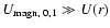
A major question arises concerning a rotating star with a magnetic field.
What happens to the meridional circulation in
presence of the magnetic field of the Tayler-Spruit dynamo? Basically, meridional
circulation occurs because thermal equilibrium cannot be achieved on
an equipotential inside a rotating star. Thus, we may wonder whether the
horizontal breakdown of thermal equilibrium in a rotating star
can be compensated by a magnetic stress
on an equipotential.
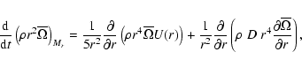
Let us define a velocity
 characterizing the radial growth of the magnetic
instability. In the two cases 0 and 1, we consider the ratio
of the appropriate maximum lengths given by
Eqs. (5) and (6) to the characteristic time
characterizing the radial growth of the magnetic
instability. In the two cases 0 and 1, we consider the ratio
of the appropriate maximum lengths given by
Eqs. (5) and (6) to the characteristic time
 ,
,
 |
(12) |
For the case 0 with
,
one
gets
 |
(13) |
Then, using the above expression (Eq. (10)) for the Alfvén frequency, we obtain
 |
(14) |
The magnetic instability grows very fastly with the angular velocity and the differential rotation parameter q.
In case 1 with
,
we get from Eq. (12) with
Eqs. (6) and (3)
 |
(15) |
Using Eq. (11) for the Alfvén frequency,
one has for the growth velocity of the magnetic instability
 |
(16) |
This velocity also grows with
and q, but less than in the case 0,
because the radiative diffusivity reduces the dependence of the
Alfvén frequency with respect to rotation parameters
and q.
These velocities have to be compared with the radial component
of the radial part of the velocity of
the meridional circulation U(r), as given by Maeder & Zahn (1998;
Eq. (4.38)). If the circulation velocity would largely dominates, this would mean that the magnetic
field has effects which are too weak to influence the meridional
circulation and the circulation would develop as usually supposed.
If on the contrary, one has
 ,
this means
that the magnetic instability develops much faster than the thermal instability
at the origin of meridional circulation.
If so, this means that the thermal instability created by rotation on an equipotential
will interact firstly with the magnetic field. Tayler
instability, which has the shortest timescale, may possibly develop
and create a magnetic field which will
introduce some stress horizontally on the equipotential.
Detailed calculations must be done with
accounting for the effects of the magnetic field in the equation for the
entropy conservation at the basis for the calculations of meridional
circulation, (this has been made for the effects of horizontal turbulence
on the meridional circulation
by Maeder & Zahn 1998).
,
this means
that the magnetic instability develops much faster than the thermal instability
at the origin of meridional circulation.
If so, this means that the thermal instability created by rotation on an equipotential
will interact firstly with the magnetic field. Tayler
instability, which has the shortest timescale, may possibly develop
and create a magnetic field which will
introduce some stress horizontally on the equipotential.
Detailed calculations must be done with
accounting for the effects of the magnetic field in the equation for the
entropy conservation at the basis for the calculations of meridional
circulation, (this has been made for the effects of horizontal turbulence
on the meridional circulation
by Maeder & Zahn 1998).
For now, we assume in this
case, in the whole region where
,
that the usual circulation velocity must be set to zero.
This working hypothesis is largely confirmed by the comparison below (cf. Tables 1 and 2)
of the velocities U(r)
of meridional circulation to the velocities
 characterizing the growth of the magnetic instability, the
last ones being 4 to 7 orders of a magnitude larger than the first one.
characterizing the growth of the magnetic instability, the
last ones being 4 to 7 orders of a magnitude larger than the first one.
Before looking more to the numerical values, we note that
some caution has to be taken so that the comparisons of
 and U(r) are done in a
consistent way. The expression
for the transfer of angular momentum
by circulation and diffusion D is (see Zahn 1992;
Maeder & Zahn 1998)
and U(r) are done in a
consistent way. The expression
for the transfer of angular momentum
by circulation and diffusion D is (see Zahn 1992;
Maeder & Zahn 1998)
 |
(17) |
where
 is the average angular velocity on the equipotential.
From the second member of this expression, we see that to any diffusion coefficient D,
one can define an associated velocity
is the average angular velocity on the equipotential.
From the second member of this expression, we see that to any diffusion coefficient D,
one can define an associated velocity 
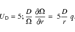 |
(18) |
The factor 5 results from the integration of the angular momentum over
the star, which leads to the above Eq. (17).
In order to be correct, the comparison of velocities
must be made over the corresponding quantities as they appear in Eq. (17)
for the angular momentum transfer,
which in turn implies Eq. (18). Now, we take the coefficients of magnetic diffusion
 and
and
 ,
which are obtained by replacing the inequalities of
Eqs. (8) and (9) by equalities. This means (cf. Spruit 2002)
that we consider the cases of marginal stability. Now, we can associate
integrated velocities to these diffusion coefficients thanks to Eq. (18)
and we find that they are just equal to the velocities
,
which are obtained by replacing the inequalities of
Eqs. (8) and (9) by equalities. This means (cf. Spruit 2002)
that we consider the cases of marginal stability. Now, we can associate
integrated velocities to these diffusion coefficients thanks to Eq. (18)
and we find that they are just equal to the velocities
 and
and
 given above multiplied by a factor of 5. These velocities characteristic
of the magnetic instability given by Eq. (18) are those to be compared to the velocity of
meridional circulation, as it appears in the equation for the transport of angular momentum.
As we shall see below, even if we omit these various considerations
about Eq. (17), which result in the above factor of 5, the conclusions
on the order of magnitude will be the same.
given above multiplied by a factor of 5. These velocities characteristic
of the magnetic instability given by Eq. (18) are those to be compared to the velocity of
meridional circulation, as it appears in the equation for the transport of angular momentum.
As we shall see below, even if we omit these various considerations
about Eq. (17), which result in the above factor of 5, the conclusions
on the order of magnitude will be the same.
Below in Sect. 6,
a star model with an initial mass of
,
a composition given by
X=0.705 and Z=0.02 and an initial rotation velocity of 300 km s-1 has been
computed. The prescriptions for rotation are those in Maeder & Meynet (2001).
Tables 1 and 2 show the main parameters when the central H-content is
 at an age of
 yr.
We see that the velocities
yr.
We see that the velocities
 are
are
 to
to
 times larger that the velocity U(r) of meridional circulation.
This shows that, even if present, the velocity of meridional circulation
is negligible with respect to the corresponding velocity characterizing the
transport of angular momentum by the magnetic field. Thus the question
whether or not meridional circulation appears in the presence of magnetic
field is of little relevance, since meridional circulation would anyway be
totally negligible in comparison of the effect of magnetic instability.
The same remark arises when one compares the magnetic
diffusion coefficients for the angular momentum as given in
Eqs. (40), (42) and (44) with the corresponding expression (28) for meridional circulation.
times larger that the velocity U(r) of meridional circulation.
This shows that, even if present, the velocity of meridional circulation
is negligible with respect to the corresponding velocity characterizing the
transport of angular momentum by the magnetic field. Thus the question
whether or not meridional circulation appears in the presence of magnetic
field is of little relevance, since meridional circulation would anyway be
totally negligible in comparison of the effect of magnetic instability.
The same remark arises when one compares the magnetic
diffusion coefficients for the angular momentum as given in
Eqs. (40), (42) and (44) with the corresponding expression (28) for meridional circulation.
Thus, we suggest that in the stellar regions where magnetic field is present,
and only there (see Sect. 5), the meridional circulation may be neglected
with respect to magnetic field effects for the transport of angular momentum.
As is shown in Sect. 4 below, the above conclusion also applies to the transport of the
chemical elements.
The turbulence in rotating stars is highly anisotropic and has a strong horizontal component,
described by a diffusion coefficient  ,
because vertically the thermal gradient stabilizes turbulence. This horizontal turbulence
strongly reduces the horizontal differential rotation, so that rotation varies only
radially. The rotation is therefore said to be "shellular'' (Zahn 1992,
uniform
at the surface of isobaric shells).
The coefficient
also plays a role in the mixing of the chemical elements and
meridional circulation (Maeder & Zahn 1998). A first expression for
was given by Zahn (1992). Recently another expression of this coefficient
has been obtained (Maeder 2003),
,
because vertically the thermal gradient stabilizes turbulence. This horizontal turbulence
strongly reduces the horizontal differential rotation, so that rotation varies only
radially. The rotation is therefore said to be "shellular'' (Zahn 1992,
uniform
at the surface of isobaric shells).
The coefficient
also plays a role in the mixing of the chemical elements and
meridional circulation (Maeder & Zahn 1998). A first expression for
was given by Zahn (1992). Recently another expression of this coefficient
has been obtained (Maeder 2003),
![$\displaystyle D_{\rm h} = A \; r \; \left[r
\overline{\Omega}(r) \; V \;
\left( 2 V - \alpha U \right)\right]^\frac{1}{3} ,$](/articles/aa/full/2003/46/aah4563/img85.gif) |
|
|
(19) |
with
 ,
V(r) the horizontal component
of meridional circulation and
,
V(r) the horizontal component
of meridional circulation and
 .
Typically, this new estimate
of
is of the order of
1011 to 1012 cm2 s-1 in a massive star,
i.e. typically 102 to 103times larger than the coefficient previously estimated. Recent
developments by Zahn (private
communication) and entered into model calculations by Palacios
(private communication) confirm this higher values of .
.
Typically, this new estimate
of
is of the order of
1011 to 1012 cm2 s-1 in a massive star,
i.e. typically 102 to 103times larger than the coefficient previously estimated. Recent
developments by Zahn (private
communication) and entered into model calculations by Palacios
(private communication) confirm this higher values of .
The question is now: what happens to this horizontal turbulence, even if it is much larger
than initially supposed,
in the presence of the magnetic field? According to Spruit (2002),
the Tayler instability and the associated dynamo leads to horizontal field
components in cases 0 and 1,
For the numerical model of Tables 1 and 2, we find an horizontal field
These fields are high with respect to our current standards,
but the magnetic pressure,
 |
(24) |
is small with respect to the total pressure. One has typically a ratio
 ,
,
 in the above
examples. Thus, the magnetic field generated by the
Tayler-Spruit mechanism does not affect the shape of the equipotentials.
The ratios
in the above
examples. Thus, the magnetic field generated by the
Tayler-Spruit mechanism does not affect the shape of the equipotentials.
The ratios
 of the radial to the horizontal field
components are given by Eqs. (21) and (23) by Spruit (2002) and
the values are of the order of 10-3 to a few 10-2.
of the radial to the horizontal field
components are given by Eqs. (21) and (23) by Spruit (2002) and
the values are of the order of 10-3 to a few 10-2.
Now, the question is how does the horizontal coupling due to the magnetic field
 compares with the horizontal turbulence characterized
by .
Spruit (2002; Eqs. (31) and (32)) has given an estimate of the coefficient
of the vertical coupling by magnetic field. However, we cannot use it here,
because the field is very anisotropic. The
coefficient
compares with the horizontal turbulence characterized
by .
Spruit (2002; Eqs. (31) and (32)) has given an estimate of the coefficient
of the vertical coupling by magnetic field. However, we cannot use it here,
because the field is very anisotropic. The
coefficient
 for the horizontal coupling must be much larger
than the vertical one. At low rotation,
we suggest to take the following estimate,
for the horizontal coupling must be much larger
than the vertical one. At low rotation,
we suggest to take the following estimate,
 |
(25) |
At high rotation, the growth rate is also reduced by the Coriolis
factor
 (as suggested by Spruit in a private communication),
thus one has then
(as suggested by Spruit in a private communication),
thus one has then
 |
(26) |
Interestingly enough, this coefficient is of the order of 1014 cm2 s-1in the above examples. Thus, the horizontal magnetic coupling is
about 103 larger than the horizontal coupling by turbulence,
even when we take the value given by the new
coefficient
in Eq. (19) above. Therefore, our conclusion
is that in the presence of Tayler-Spruit dynamo, we can anyway neglect the
coupling due to horizontal turbulence with respect to the coupling insured by
the horizontal component of the magnetic field. More likely, we
suspect that the horizontal turbulence may not develop in this case or occur in a very
different and limited way.
In models with rotation and without magnetic fields, the combined effect
of meridional circulation and horizontal turbulence may be treated
as a diffusion with a coefficient usually called
 (cf. Chaboyer & Zahn 1992),
![\begin{displaymath}D_{\rm eff}= \frac{\left[r\; U(r)\right]^2}{30 \; D_{\rm h}} \cdot
\end{displaymath}](/articles/aa/full/2003/46/aah4563/img104.gif) |
(27) |
Now, since
is negligible, we may wonder what happens
to the transport of chemical elements by meridional circulation.
As well known, it is in general not correct to express an advection
as a diffusion, but let us do it here just for the purpose of comparing
orders of magnitude. The diffusion coefficient we may associate
to the meridional circulation is in this case,
 |
(28) |
This must be compared to the coefficients
 ,
which are obtained by imposing equality in Eqs. (8) and (9)
and taking
,
which are obtained by imposing equality in Eqs. (8) and (9)
and taking
 .
The equality
means that one considers the case of marginal stability as determining for
the transport.
Then, in the obtained
relations, the Alfvén frequency is expressed with the help
of Eqs. (10) and (11). In this way, Spruit obtains
(2002; Eqs. (42) and (43)),
.
The equality
means that one considers the case of marginal stability as determining for
the transport.
Then, in the obtained
relations, the Alfvén frequency is expressed with the help
of Eqs. (10) and (11). In this way, Spruit obtains
(2002; Eqs. (42) and (43)),
 |
(29) |
and
 |
(30) |
In the numerical example of Tables 1 and 2, we find ratios
 ,
,
 ,
,
 at the 3 layers considered, (taking in each case the appropriate
expressions for the case 0 and 1). Thus, we see that through most
of the star the circulation (if it exists!) would have a negligible effect for the transport
of chemical elements. Only close to the
core, the circulation
might represent about 10% of the transport by the magnetic instability.
This is small anyway and owing to the profound doubts expressed above on the
occurrence
of any circulation, we consider that any transport of chemical elements by
meridional circulation can generally be neglected in the presence of
Tayler-Spruit dynamo.
at the 3 layers considered, (taking in each case the appropriate
expressions for the case 0 and 1). Thus, we see that through most
of the star the circulation (if it exists!) would have a negligible effect for the transport
of chemical elements. Only close to the
core, the circulation
might represent about 10% of the transport by the magnetic instability.
This is small anyway and owing to the profound doubts expressed above on the
occurrence
of any circulation, we consider that any transport of chemical elements by
meridional circulation can generally be neglected in the presence of
Tayler-Spruit dynamo.
In a radiative zone, the magnetic field created by the Tayler-Spruit instability arises
from differential rotation.
Therefore, we must impose the condition that the
energy in the magnetic field cannot be larger than the excess energy in differential
rotation. Tayler (1973) and Pitts & Tayler (1986) have
studied the conditions for the appearance of the magnetic instabilities,
which have very short growth times. The above condition is different, it is an
energy condition, which must be satisfied on longer timescales.
Due to the magnetic diffusivity, the field once created tends to disappear.
Taking the values of
 given for example in Fig. 6 (see also Tables 1 and 2), which are between 1010.5 and 1012 cm2 s-1 over most of the star except very close to the convective
core, we find that the timescale
given for example in Fig. 6 (see also Tables 1 and 2), which are between 1010.5 and 1012 cm2 s-1 over most of the star except very close to the convective
core, we find that the timescale
 for the diffusion of the magnetic field is of the order of
 to
to
 yr, which is short with respect to the
stellar lifetimes. This means that the field created by Tayler-Spruit dynamo
will exist only if the energy of the magnetic field is
continuously replenished by differential rotation during the MS evolution. Therefore, we
need to apply the above condition.
yr, which is short with respect to the
stellar lifetimes. This means that the field created by Tayler-Spruit dynamo
will exist only if the energy of the magnetic field is
continuously replenished by differential rotation during the MS evolution. Therefore, we
need to apply the above condition.
For a magnetic instability with a displacement
of amplitude  ,
the kinetic energy EB by unit of mass is
,
the kinetic energy EB by unit of mass is
 |
(31) |
The excess energy
 in the differential rotation is the difference of energy
between the existing flow with differential rotation and a flow with an average rotation over the
considered radial distance r. Let us consider
a horizontal velocity field W(r). Over a vertical distance dr, the
energy excess d
over the extent of the magnetic instability is
in the differential rotation is the difference of energy
between the existing flow with differential rotation and a flow with an average rotation over the
considered radial distance r. Let us consider
a horizontal velocity field W(r). Over a vertical distance dr, the
energy excess d
over the extent of the magnetic instability is
If  and
and  are the
radial and horizontal components of the displacement
of the magnetic oscillation
(cf. Spruit 2002), the energy excess over the displacement
can be written,
are the
radial and horizontal components of the displacement
of the magnetic oscillation
(cf. Spruit 2002), the energy excess over the displacement
can be written,
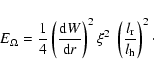 |
(33) |
The horizontal velocity
 ,
where
,
where  is the colatitude.
Thus, one has
is the colatitude.
Thus, one has
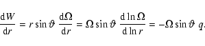 |
(34) |
The condition
 leads to
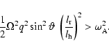 |
(35) |
This would apply to a given colatitude .
This equation
as it stands means that the reservoir of
available rotational energy is larger at the equator, while we know (cf. Spruit
1999) on the other hand that Tayler instability is stronger away from equator.
Now, for the ratio
 of the vertical to the horizontal displacement, we could take for example in the outer
layers, where differential rotation is generally small, the value given by Eq. (6)
above (case 1). This promptly leads to the following criterion
with account of Eq. (11),
of the vertical to the horizontal displacement, we could take for example in the outer
layers, where differential rotation is generally small, the value given by Eq. (6)
above (case 1). This promptly leads to the following criterion
with account of Eq. (11),
 |
(36) |
This equation ignores the geometry of the field.
However, we have to consider carefully
the geometry of the problem in 2 specific respects:
1. We must account for the
fact that in the model of shellular rotation
the energy of rotation is not a local quantity depending on
 ,
but on r only. The physical reason in the usual rotating models is
the strong horizontal turbulence (cf. Zahn 1992). In the present models,
the horizontal magnetic coupling is even stronger, as seen above in Sect. 4.1, so that
shellular rotation is a valid assumption here. In such a case,
the average stellar structure of the rotating star
corresponds very well to the structure at a colatitude
given by
the root of the second
Legendre polynomial
,
but on r only. The physical reason in the usual rotating models is
the strong horizontal turbulence (cf. Zahn 1992). In the present models,
the horizontal magnetic coupling is even stronger, as seen above in Sect. 4.1, so that
shellular rotation is a valid assumption here. In such a case,
the average stellar structure of the rotating star
corresponds very well to the structure at a colatitude
given by
the root of the second
Legendre polynomial
 ,
(this has been verified in a recent work, Maeder 2001). Thus it is appropriate to consider for the differential rotation
,
(this has been verified in a recent work, Maeder 2001). Thus it is appropriate to consider for the differential rotation
 in Eq. (34) on a given equipotential
the average value
in Eq. (34) on a given equipotential
the average value
 .
.
2. The geometry of the field is also particular (cf. Spruit 1999,2002).
It consists of stacks of magnetic loops concentric with the rotation axis.
The main component of the displacement due to the Tayler instability
is perpendicular to the rotation axis. This means that at colatitude
,
the ratio
behaves
essentially as
 .
Since the polar caps are most unstable, while the
equatorial regions are not, it is
clear that in the polar regions one has a ratio
smaller than 1.
However, in 1D models as here we must consider the significant average
for the whole range of colatitudes. The field behaves as
.
Since the polar caps are most unstable, while the
equatorial regions are not, it is
clear that in the polar regions one has a ratio
smaller than 1.
However, in 1D models as here we must consider the significant average
for the whole range of colatitudes. The field behaves as
 (cf. Spruit 1999; Eq. (35)) and the Tayler instability develops only for
 ,
therefore
it is necessary on a given isobar to consider colatitudes
smaller or
at most equal to
,
therefore
it is necessary on a given isobar to consider colatitudes
smaller or
at most equal to  .
If we take this last value as the limit, this gives the upper
bound
.
If we take this last value as the limit, this gives the upper
bound
 .
.
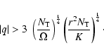
From these two geometrical remarks, we obtain
the necessary condition for the existence
of a magnetic field generated by the Tayler-Spruit dynamo as follows,
 |
(37) |
This means that the degree of differential rotation q must at least be larger
than  times the ratio
of the Alfvén to the rotation frequency, in order that there is enough
energy in the differential rotation to allow the Tayler-Spruit dynamo
to operate and build a magnetic field. We insist that this is a necessary condition.
If this condition is not realized, there
is certainly no magnetic field created by the dynamo. Further work may perhaps
lead to an even more constraining condition.
The numerical factor, here ,
may depend on the exact geometry of the magnetic displacements in a rotating star.
We note also that
if there are several types of instabilities generated by differential
rotation, the available energy given by Eq. (33) would in some way be
shared between the instabilities. However, as mentioned above, the Tayler instability is
the main one and shear instabilities appear negligible in comparison.
times the ratio
of the Alfvén to the rotation frequency, in order that there is enough
energy in the differential rotation to allow the Tayler-Spruit dynamo
to operate and build a magnetic field. We insist that this is a necessary condition.
If this condition is not realized, there
is certainly no magnetic field created by the dynamo. Further work may perhaps
lead to an even more constraining condition.
The numerical factor, here ,
may depend on the exact geometry of the magnetic displacements in a rotating star.
We note also that
if there are several types of instabilities generated by differential
rotation, the available energy given by Eq. (33) would in some way be
shared between the instabilities. However, as mentioned above, the Tayler instability is
the main one and shear instabilities appear negligible in comparison.
We can go a step further, since the Alfvén frequency
is a function of rotation and differential parameter |q|.
For the case 0, where the -gradient dominates,
the ratio
is given by the above Eq. (10). Thus, the above condition (37)
becomes in this case
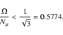 |
(38) |
This is the necessary condition in order that a magnetic field may develop
from differential rotation in case 0. At first glance, this condition
may look strange, since it means that
must be smaller that some value.
The reason is that
grows like
 ,
while the upper limiting
expressed by Eq. (37)
goes like
,
while the upper limiting
expressed by Eq. (37)
goes like
 .
Thus, if would be too big, the actual
would overcome the critical value.
In the numerical examples of Tables 1 and 2,
case 0 is relevant at the edge of the core
at
.
Thus, if would be too big, the actual
would overcome the critical value.
In the numerical examples of Tables 1 and 2,
case 0 is relevant at the edge of the core
at
 .
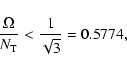
There
.
There
 is 0.11, (typically
lies between 0.1 and 0.15
throughout the star). This is smaller than
0.5774 and thus the magnetic field can be present in these layers.
is 0.11, (typically
lies between 0.1 and 0.15
throughout the star). This is smaller than
0.5774 and thus the magnetic field can be present in these layers.
We now consider case 1 with thermal diffusion, the Alfvén frequency
is given by Eq. (11). With the above condition (37), one obtains
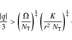 |
(39) |
This means that the differential rotation parameter |q| has to be large enough
to be able to generate the magnetic field. In the numerical examples in Sect. 6,
the condition is not satisfied in the very outerlayers, which have a too weak
differential rotation.
![\begin{figure}
\par\includegraphics[width=8cm,clip]{fx.eps}
\end{figure}](/articles/aa/full/2003/46/aah4563/Timg150.gif) |
Figure 1:
Internal H-profile in the
test model with
km s-1.
The model is
at an age of
 yr. This is the reference model in which
we examine the properties of the magnetic field in detail. yr. This is the reference model in which
we examine the properties of the magnetic field in detail. |
| Open with DEXTER |
Let us collect here the various expressions we have for the
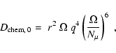
diffusion coefficients by the Tayler-Spruit dynamo in radiative zones.
Case 0 applies when
.
Magnetic field is
present only when the criterion given by Eq. (38) is satisfied. Then
the diffusion coefficients for the transport of the angular momentum
and chemical elements are respectively,
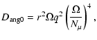 |
|
|
(40) |
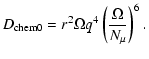 |
|
|
(41) |
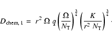
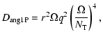
Case 1 applies when
,
then account is given to the thermal
diffusivity. Magnetic field is
present only when the criterion given by Eq. (39) is satisfied.
The diffusion coefficients for the angular
momentum and chemical elements are respectively
 |
|
|
(42) |
 |
|
|
(43) |
Normally, these coefficients are larger than those which would be obtained in case 0
with  instead of ,
because
the account for thermal effects reduces the buoyancy force which opposes to the
magnetic instability. However, as noted by Spruit (2002), it may happen
in some cases that these
coefficients with index "1'' are smaller. As noted by Spruit (2002),
this is an artefact from the simplification introduced by
considering only the 2 limiting cases 0 and 1. Spruit
suggests to introduce an interpolation formula depending on q. We hesitate to do so,
because this extra-dependence on the differential rotation parameter q is unphysical,
since the interpolation should rather depend on the thermal and magnetic diffusivities K and .
Thus, the suggested treatment might
introduce spurious effects in some evolutionary stages. The general case where thermal
effects and -gradient are accounted for needs to be worked out
in future. For now, we prefer to do the following by considering
the coefficients
instead of ,
because
the account for thermal effects reduces the buoyancy force which opposes to the
magnetic instability. However, as noted by Spruit (2002), it may happen
in some cases that these
coefficients with index "1'' are smaller. As noted by Spruit (2002),
this is an artefact from the simplification introduced by
considering only the 2 limiting cases 0 and 1. Spruit
suggests to introduce an interpolation formula depending on q. We hesitate to do so,
because this extra-dependence on the differential rotation parameter q is unphysical,
since the interpolation should rather depend on the thermal and magnetic diffusivities K and .
Thus, the suggested treatment might
introduce spurious effects in some evolutionary stages. The general case where thermal
effects and -gradient are accounted for needs to be worked out
in future. For now, we prefer to do the following by considering
the coefficients
 |
|
|
(44) |
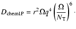 |
|
|
(45) |
These are the same equations as in case 0, but with
instead of .
This means that we are considering only the restoring force of the thermal gradient
and that we are ignoring the non-adiabatic radiative losses.
![\begin{figure}
\par\includegraphics[width=8cm,clip]{fn.eps}
\end{figure}](/articles/aa/full/2003/46/aah4563/Timg158.gif) |
Figure 2:
The oscillation frequencies in the model of Fig. 1.
 is indicated by a continuous line and
 is given
by a dashed line.
is given
by a dashed line. |
| Open with DEXTER |
For case 1, we compare the coefficient with indices "1'' and "1P''
and must take the larger ones. From Fig. (5) below, we see that the coefficients "1P'' may be larger than the coefficients "1''
in some parts of the star. Of course, we have also to test whether
the magnetic field can be created from differential rotation. For such zones of case 1P, the
criterion for the existence of the magnetic field is evidently the following one
 |
(46) |
and the appropriate test has to be made in the concerned layers.
We calculate evolutionary models of a
star with initial composition
X=0.705 and Z=0.02. The physics of the models (opacities, nuclear reactions, mass loss rates,
treatment of rotation, increase of the mass loss rates with rotation, etc.)
are the same as in Meynet & Maeder (2003).
We compute the MS evolution of a model with
an initial velocity of 300 km s-1, which leads to an average velocity during the MS phase
of about 220 km s-1, which corresponds to the observed average rotation velocity.
We now consider in detail the properties of a particular model with rotation to see
the various coefficients and criteria characterizing the growth
of the magnetic field.
We take the model at an age
yr with a central
H-content
.
The H-profile inside the star is illustrated in
Fig. 1 and the oscillation frequencies
and
in Fig. 2. We see that case 0 applies between
 and 1.59, which corresponds to mass coordinates
5.53 and
and 1.59, which corresponds to mass coordinates
5.53 and
 respectively. The internal profile
  is illustrated
in Fig. 3.
is illustrated
in Fig. 3.
![\begin{figure}
\par\includegraphics[width=8cm,clip]{fom.eps}
\end{figure}](/articles/aa/full/2003/46/aah4563/Timg162.gif) |
Figure 3:
The distribution of the angular velocity in the reference model of Fig. 1
with rotation (continuous line). |
| Open with DEXTER |
![\begin{figure}
\par\includegraphics[width=8cm,clip]{fd.eps}
\end{figure}](/articles/aa/full/2003/46/aah4563/Timg163.gif) |
Figure 4:
The diffusion coefficients
 (continuous line) and
 (dashed line) corresponding to case 0. As discussed in the text,
these coefficients apply only in the rising
part between
and 1.59.
(dashed line) corresponding to case 0. As discussed in the text,
these coefficients apply only in the rising
part between
and 1.59. |
| Open with DEXTER |
The diffusion coefficients
and
are illustrated
in Fig. 4. These coefficients grow very fastly at the edge of the core
since
decreases very fastly there and the dependence in the ratio
 goes like the power 4 and 6 for the two coefficients
respectively. These coefficients apply only in the rising
part between
and 1.59 as indicated. Above this value, the main
restoring force is no longer the -gradient, but the stable temperature gradient.
goes like the power 4 and 6 for the two coefficients
respectively. These coefficients apply only in the rising
part between
and 1.59 as indicated. Above this value, the main
restoring force is no longer the -gradient, but the stable temperature gradient.
![\begin{figure}
\par\includegraphics[width=8cm,clip]{fd2.eps}
\end{figure}](/articles/aa/full/2003/46/aah4563/Timg165.gif) |
Figure 5:
The diffusion coefficients for angular momentum
 (continuous line)
and
(continuous line)
and
 (dotted line). The diffusion coefficients for chemical
elements
(dotted line). The diffusion coefficients for chemical
elements
 (dashed line) and
 (long dashed line).
In each case, the largest diffusion coefficient has to be taken.
(long dashed line).
In each case, the largest diffusion coefficient has to be taken. |
| Open with DEXTER |
In case 1, where thermal gradients dominate, the diffusion coefficients are
illustrated in Fig. 5. We see that for the transports of
angular momentum and of chemical elements, the coefficients with indices "1''
dominate in the external parts of the star above
 .
However, we also notice that in a sizeable
region, i.e. between
.
However, we also notice that in a sizeable
region, i.e. between
 and 2.69,
the coefficients with indices "
and 2.69,
the coefficients with indices "
 '' dominate
over those with "1''. This occurs, as expected, at some limited
distance above the edge of the convective core, at the place where the -gradient
becomes small enough, but is still different from zero. In these regions, more general developments
having case 0 and 1 as limiting cases would be a progress. We see that the differences between
the two cases "
'' and "1'' amounts to a maximum of 0.4 dex and 0.6 dex
for the transport of angular momentum and chemical elements respectively. This is limited, but
non negligible, and it may justify a further study of the physics of the
general case. However, we notice that this difference is small when compared
to the differences resulting from the inclusion of the magnetic field
or not, which as shown below amounts to several orders of magnitude.
Thus, we conclude that the present coefficients of diffusion
need to be further improved, but they nevertheless describe correctly the
main results of the inclusion of the magnetic field.
'' dominate
over those with "1''. This occurs, as expected, at some limited
distance above the edge of the convective core, at the place where the -gradient
becomes small enough, but is still different from zero. In these regions, more general developments
having case 0 and 1 as limiting cases would be a progress. We see that the differences between
the two cases "
'' and "1'' amounts to a maximum of 0.4 dex and 0.6 dex
for the transport of angular momentum and chemical elements respectively. This is limited, but
non negligible, and it may justify a further study of the physics of the
general case. However, we notice that this difference is small when compared
to the differences resulting from the inclusion of the magnetic field
or not, which as shown below amounts to several orders of magnitude.
Thus, we conclude that the present coefficients of diffusion
need to be further improved, but they nevertheless describe correctly the
main results of the inclusion of the magnetic field.
![\begin{figure}
\par\includegraphics[width=8cm,clip]{fdi.eps}
\end{figure}](/articles/aa/full/2003/46/aah4563/Timg168.gif) |
Figure 6:
The figure shows the complete description
of the diffusion coefficient
 for angular momentum (continuous line) made according to prescriptions of Sect. 5.2. The complete description of the diffusion coefficient
 for chemical elements is given by the dashed line.
The dotted line shows the shear diffusion coefficient
for chemical elements is given by the dashed line.
The dotted line shows the shear diffusion coefficient
 from Maeder (1997). The thermal diffusivity coefficient K is represented
by a long-dashed line.
from Maeder (1997). The thermal diffusivity coefficient K is represented
by a long-dashed line. |
| Open with DEXTER |
Tables 1 and 2 provides some useful structural parameters, the
diffusion coefficients and the velocities of meridional circulation and of magnetic
instability at 3 locations
in the reference model of
with
an initial velocity of 300 km s-1 at an age
yr.
The three levels considered illustrate the case 0,
1P and 1 respectively. These Tables permit further quantitative analysis
of the various terms intervening in the equations.
Figure 6 shows the comparison of the diffusion coefficients due
to the magnetic field compared to the diffusion coefficient
by shear
instability in the rotating star and to the thermal diffusivity K.
The transport of angular momentum by the
magnetic field is 6-7 orders of magnitude stronger than by shear instability in a rotating star.
Similarly, as discussed in Sect. 4.2, the magnetic transport of angular momentum
is also 4-7 orders of magnitude larger than by meridional circulation. Therefore, we conclude
that transport of angular momentum by magnetic field is totally dominating, if magnetic field is present.
For the transport of chemical elements, the difference between the two diffusion coefficients
amount to 3-5 orders of magnitude in favour of the transport by magnetic field. The
difference is especially large in deep regions at some distance of
the convective core. At the very edge of the convective core,
the dependence of the coefficient
 in the power 6 of
reduces the magnetic diffusion
drastically, so that as mentioned in Sect. 4.2 the ratio
of the transport of chemical elements by the magnetic instability to the transport by
circulation may amount to about 1 order of magnitude.
Some tests indicate that this makes the chemical enrichments in helium and nitrogen at the
stellar surface are stronger, but not too different,
from those without magnetic field, despite the fact that
the diffusion coefficients with magnetic field are orders
of magnitude larger over most of the stellar interior.
On the whole, we see that for chemical mixing also, the magnetic
instability plays a great role.
in the power 6 of
reduces the magnetic diffusion
drastically, so that as mentioned in Sect. 4.2 the ratio
of the transport of chemical elements by the magnetic instability to the transport by
circulation may amount to about 1 order of magnitude.
Some tests indicate that this makes the chemical enrichments in helium and nitrogen at the
stellar surface are stronger, but not too different,
from those without magnetic field, despite the fact that
the diffusion coefficients with magnetic field are orders
of magnitude larger over most of the stellar interior.
On the whole, we see that for chemical mixing also, the magnetic
instability plays a great role.
It is also interesting to see that diffusion coefficients by the magnetic field
are almost equal (transport of chemical elements) or even larger
(transport of the angular momentum) than the thermal diffusivity.
This means that magnetic effects by the Tayler-Spruit dynamo
are in general equal or larger than thermal effects. Globally thermal
effects may be relatively more significant in the outer layers.
An important question in the models is to determine at each shell mass
whether differential rotation described by parameter qis sufficient to create the Tayler-Spruit dynamo
to produce a magnetic field. We examine here whether these conditions are
fulfilled in the model with rotation only studied in the previous
subsection. Firstly, we examine the regions adjacent
to the core between
and 1.59,
where case 0 applies, since
dominates.
Figure 7 shows the difference
 ,
we see that in the concerned region between
and 1.59,
this difference is negative, thus magnetic field is present there. This is an interesting result
because it means that despite the strong restoring buoyancy force due to the
very large -gradient, the differential rotation is high enough to
develop magnetic instability.
At each time step during evolution, such tests need to be performed.
,
we see that in the concerned region between
and 1.59,
this difference is negative, thus magnetic field is present there. This is an interesting result
because it means that despite the strong restoring buoyancy force due to the
very large -gradient, the differential rotation is high enough to
develop magnetic instability.
At each time step during evolution, such tests need to be performed.
![\begin{figure}
\par\includegraphics[width=8cm,clip]{onmu.eps}
\end{figure}](/articles/aa/full/2003/46/aah4563/Timg171.gif) |
Figure 7:
The difference
when case 0 applies,
i.e. in the region between
and 1.59.
According to criterion (38), if this difference is negative,
magnetic field is created. Thus, we see that in the region where the -gradient
dominates, magnetic field can be generated by the Tayler-Spruit dynamo. |
| Open with DEXTER |
Secondly, we examine the zone above
and up to
,
where case 1P applies. There, we check for the difference
 .
If this expression is negative,
magnetic field is created. This expression lies between
-0.40 and -0.50 in this whole intermediate region. Thus, we conclude that
magnetic field is also present there.
.
If this expression is negative,
magnetic field is created. This expression lies between
-0.40 and -0.50 in this whole intermediate region. Thus, we conclude that
magnetic field is also present there.
The criterion for the existence of the magnetic field in the external zone,
which corresponds to case 1 is given by Eq. (39). From Fig. 8,
we see that in this zone
which lies between
 and the surface, the difference
 is generally
positive, which means that magnetic field is present over that region. However,
we notice that very close to the surface this difference goes to zero. This means
that at the surface, differential rotation is becoming insufficient to generate the
magnetic instability. This is interesting because it may explain why there is in general no
strong magnetic field observed at the surface of OB stars (cf. Mathys 2003), despite
the likely existence of a strong internal field created the Tayler-Spruit instability.
is generally
positive, which means that magnetic field is present over that region. However,
we notice that very close to the surface this difference goes to zero. This means
that at the surface, differential rotation is becoming insufficient to generate the
magnetic instability. This is interesting because it may explain why there is in general no
strong magnetic field observed at the surface of OB stars (cf. Mathys 2003), despite
the likely existence of a strong internal field created the Tayler-Spruit instability.
![\begin{figure}
\par\includegraphics[width=8cm,clip]{ontt.eps}
\end{figure}](/articles/aa/full/2003/46/aah4563/Timg176.gif) |
Figure 8:
The quantity
 given by Eq. (39) vs.
 .
When this quantity is positive in the region where case 1 applies, i.e.
above
,
differential rotation is sufficient to generate the magnetic
field, which is the case here. .
When this quantity is positive in the region where case 1 applies, i.e.
above
,
differential rotation is sufficient to generate the magnetic
field, which is the case here. |
| Open with DEXTER |
These results show that in a rotating star,
the conditions on the differential rotation for the growth of
the magnetic field are largely realized, with the
possible exception of the superficial layers.
The main conclusion is that the Tayler instability and the Tayler-Spruit dynamo
are of major
importance for stellar evolution, both for the transport of angular momentum and
for the transport of chemical elements. Future evolutionary models applying
the results of this work will be made to study
the results on tracks, surface composition, rotation, etc.
It is likely that in a rotating star calculated with magnetic field from the beginning,
the differential rotation is very much reduced by the magnetic transport
of angular momentum described above. We may suspect that differential
rotation will be reduced down to a stage where the criterion (37) discussed
in Sect. 5.1 is just marginally satisfied, i.e.
 |
(47) |
Indeed, if differential rotation is higher than given by this criterion, magnetic field
develops and the associated coupling reduces differential rotation.
If, at the opposite, differential rotation is lower
than given by criterion (47), the growth of mean molecular weight by nuclear reactions in the central regions together with angular momentum conservation will produce an
enhancement of differential rotation. Thus, a stage of marginal equilibrium
is most likely reached during MS evolution. It may also be that the outer layers
never have sufficient differential rotation to build Tayler-Spruit dynamo.
Further numerical models will explore the evolution of stars with rotation and magnetic field, and
analyse the coupling between magnetic field and differential rotation.
Note added in proof: The above calculations determine the magnetic field
which develops
in a rotating star, which had no field until a considered specific evolutionary stage.
Recent calculations have confirmed, as suggested in the conclusions, that models with
magnetic field included throughout MS evolution reach an equilibrium situation with
very little differential rotation. This happens in turn to make a feedback on the field
amplitude and on the velocity of meridional circulation. This has two consequences:
a) the internal magnetic fields are reduced to a few 104 G; b) the velocity of meridional
circulation is increased to about
 .
This confirms that magnetic fields
play an essential role. However, in the equilibrium models some effects
of meridional circulation could also influence the internal profile of
due to the above feedback.
.
This confirms that magnetic fields
play an essential role. However, in the equilibrium models some effects
of meridional circulation could also influence the internal profile of
due to the above feedback.
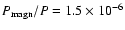
Acknowledgements
We express our best thanks to Dr. H.C. Spruit for very useful comments.
The most valuable remarks of an unknown referee are also acknowledged with thanks.
-
Chaboyer, B., & Zahn, J.-P. 1992, A&A, 253, 173
In the text
NASA ADS
-
Langer, N., Heger, A., Wellstein, S., & Herwig, F. 1999, A&A, 346, 37L
In the text
NASA ADS
-
Maeder, A. 1997, A&A, 321, 134
In the text
NASA ADS
-
Maeder, A. 2001, A&A, 373, 122
In the text
NASA ADS
-
Maeder, A. 2003, A&A, 399, 263
In the text
NASA ADS
-
Maeder, A., & Meynet, G. 2000, ARA&A, 38, 143
In the text
NASA ADS
-
Maeder, A., & Meynet, G. 2001, A&A, 373, 555 (Paper VII)
In the text
NASA ADS
-
Maeder, A., & Zahn, J. P. 1998, A&A, 334, 1000 (Paper III)
In the text
NASA ADS
-
Mathys, G. 2003, in Stellar Rotation, IAU Symp. 215, ed. A. Maeder, & P. Eenens,
ASP Conf. Ser. in press
In the text
-
Meynet, G., & Maeder, A. 2003, A&A, 404, 975 (Paper X)
In the text
NASA ADS
-
Pitts, E., & Tayler, R. J. 1986, MNRAS, 216, 139
In the text
-
Spruit, H. C. 1999, A&A, 349, 189
In the text
NASA ADS
-
Spruit, H. C. 2002, A&A, 381, 923
In the text
NASA ADS
-
Tayler, R. J. 1973, MNRAS, 161, 365
In the text
NASA ADS
-
Zahn, J. P. 1992, A&A, 265, 115
In the text
NASA ADS
Copyright ESO 2003
![$\displaystyle \frac{1}{2} \left[ W^2 + (W+{\rm d}W)^2 \right] -\frac{1}{2} \cdot 2
\left(W+\frac{{\rm d}W}{2}\right)^2$](/articles/aa/full/2003/46/aah4563/img121.gif)
![\begin{figure}
\par\includegraphics[width=8cm,clip]{fx.eps}
\end{figure}](/articles/aa/full/2003/46/aah4563/img150.gif)
![\begin{figure}
\par\includegraphics[width=8cm,clip]{fn.eps}
\end{figure}](/articles/aa/full/2003/46/aah4563/img158.gif)
![\begin{figure}
\par\includegraphics[width=8cm,clip]{fom.eps}
\end{figure}](/articles/aa/full/2003/46/aah4563/img162.gif)
![\begin{figure}
\par\includegraphics[width=8cm,clip]{fd.eps}
\end{figure}](/articles/aa/full/2003/46/aah4563/img163.gif)
![\begin{figure}
\par\includegraphics[width=8cm,clip]{fd2.eps}
\end{figure}](/articles/aa/full/2003/46/aah4563/img165.gif)
![\begin{figure}
\par\includegraphics[width=8cm,clip]{fdi.eps}
\end{figure}](/articles/aa/full/2003/46/aah4563/img168.gif)
![\begin{figure}
\par\includegraphics[width=8cm,clip]{onmu.eps}
\end{figure}](/articles/aa/full/2003/46/aah4563/img171.gif)
![\begin{figure}
\par\includegraphics[width=8cm,clip]{ontt.eps}
\end{figure}](/articles/aa/full/2003/46/aah4563/img176.gif)