E. Ya. Zlotnik1 - V. V. Zaitsev1 - H. Aurass2 - G. Mann2 - A. Hofmann2
1 - Institute of Applied Physics RAS, 603600 Nizhny Novgorod, Russia
2 -
Astrophysical Institute Potsdam, 14482 Potsdam, Germany
Received 2 June 2003 / Accepted 28 July 2003
Abstract
We discuss a
source model for the origin of solar type IV burst fine structures
(FS) using the data of an event in AR 7792 on 25 October 1994.
After giving a comprehensive observational treatment of FS (Paper
I), here we repeat the main observed facts to construct a
simplified radio source model. It consists of two interacting
loops (named LS1 and EL) with one spatial order of magnitude scale
difference (turning heights 70 and 7 Mm). We consider the
implications of this model for physical mechanisms of broad band
pulsations (BBP) and zebra patterns (ZP). Our analysis
leads to the conclusion that meter wave BBP and ZP originate from
a common magnetic source structure - a large asymmetric coronal
loop. It is shown that the BBP result from periodically repeated
injections of fast electrons into the asymmetric magnetic trap.
The excitation of plasma waves is due to the stream instability
when these electrons are propagating along the loop. We
demonstrate that a two percent quasi-periodic modulation of a
magnetic field component in EL is sufficient for it to act as a
periodic electron accelerator. The ZP is due to a plasma wave
instability at the levels of double plasma resonance (DPR) in an
inhomogeneous source distributed along the loop axis of LS1. The
DPR frequencies appear at those height levels where the upper
hybrid frequency is equal to a harmonic of the gyrofrequency. Two
Appendices review theoretical details needed to understand the
given ZP interpretation. The gyrofrequency as a function of height
was derived from a force-free extrapolated field line that passes
the coronal radio source. After knowing the loop turning height
and the magnetic field strength we identified for a fixed
observing time the harmonic number of each zebra stripe. The
comparison of the calculated DPR levels with the observed zebra
stripe peak frequencies yields a density law for the ZP source
volume. It turns out that this is a barometric law with a
temperature near 106 K. We demonstrate that the drift of the
whole ZP to higher frequencies can be explained as a signature of
magnetic field decrease and/or plasma cooling in the ZP source.
The time delay between BBP and ZP was found to be due to the
higher fast particle threshold of the DPR versus the beam
instability. The present analysis confirms the double plasma
resonance model for the ZP fine structure, and underlines the
significance of force-free extrapolated photospheric fields for
coronal magnetic field modelling.
Key words: Sun: flares - Sun: corona - Sun: radio radiation - Sun: magnetic fields
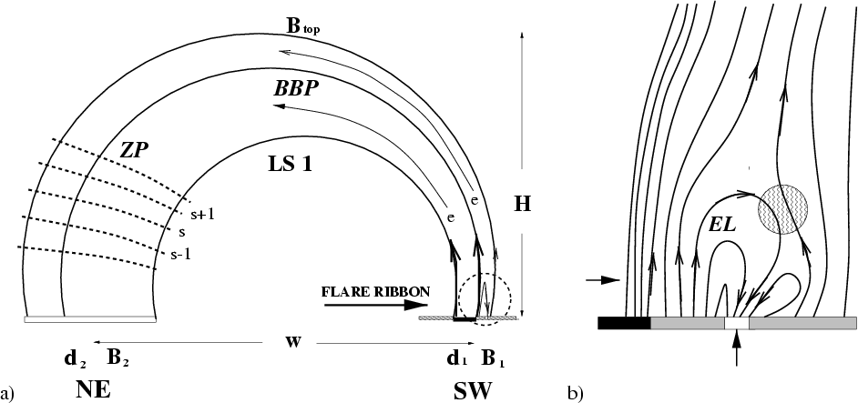 |
Figure 1: Source model from optical, X-ray and radio measurements (see Paper I). a) The loop LS1 is the main source of BBP and ZP: fast electron streams exciting BBP are injected at the SW footpoint. ZP stripes arise at the DPR levels (stippled) in the NE part of LS1. b) Enlargement of the encircled SW range: the leading spot in conflict with the emerging parasitic polarity loop (EL). The wavy circle is a site of reconnection and electron acceleration. |
| Open with DEXTER | |
In Paper I, we gave an extended introduction to the problem of solar radio burst
continuum fine structures (FS) with special regard to broad band pulsations
(BBP) and zebra patterns (ZP). There, the reader can find detailed reference to
earlier work in the field. Paper I presents the FS observations for the event of
October 25, 1994 in active region NOAA 7792 and explains (together with Aurass
et al. 1999) the relation between the radio data and the magnetic field
measurements in the photosphere, its extrapolation to the corona, and to the
Yohkoh soft X-ray and the H![]() imaging data. Here we briefly
summarize the data directly related to the occurrence of radio pulsations and
zebra patterns and which can elucidate the most probable reasons of their
origin.
imaging data. Here we briefly
summarize the data directly related to the occurrence of radio pulsations and
zebra patterns and which can elucidate the most probable reasons of their
origin.
Using the observational data and bearing in mind our interpretation of BBP and
ZP in the event of interest, we plotted in Fig. 1 a simplified
outline of a source model thereby sketching the origin of the observed
FS. The main source of BBP and ZP is located in a highly asymmetric loop
forming a magnetic trap. Magnetic field
strengths at the loop footpoints were
![]() G and
G and
![]() G. The diameters of footpoint regions were taken as
G. The diameters of footpoint regions were taken as
![]() Mm and
Mm and
![]() Mm, correspondingly. The distance between
footpoints was
Mm, correspondingly. The distance between
footpoints was
![]() Mm. The loop extended up to
Mm. The loop extended up to
![]() Mm
above the photosphere, and the average magnetic field at the
top of the trap was
Mm
above the photosphere, and the average magnetic field at the
top of the trap was
![]() G. The source of fast electrons
was concentrated near the footpoint d1with strong magnetic field B1. We know that the interaction of a small-scale
loop system saturating emerging parasitic flux with the loop systems LS1 and LS2
(Fig. 2 of Paper I, and Aurass et al. 1999) is driven during the flare. The
accelerated electrons were moving along the trap axis from its footpoint to the
top. We suggest that the fast electrons
arise either due to the interaction of the asymmetric loop LS1 with emerging
flux EL, or due to processes inside the compact loop EL with following injection
into the big trap LS1.
G. The source of fast electrons
was concentrated near the footpoint d1with strong magnetic field B1. We know that the interaction of a small-scale
loop system saturating emerging parasitic flux with the loop systems LS1 and LS2
(Fig. 2 of Paper I, and Aurass et al. 1999) is driven during the flare. The
accelerated electrons were moving along the trap axis from its footpoint to the
top. We suggest that the fast electrons
arise either due to the interaction of the asymmetric loop LS1 with emerging
flux EL, or due to processes inside the compact loop EL with following injection
into the big trap LS1.
According to radio imaging data (see Paper I), the ZP source was localized in the region of a weak magnetic field in the trap LS1 (d2), while the BBP source was closer to the footpoint with a strong magnetic field (d1). We will argue that the BBP in the considered event are associated with fast electron beams, periodically injected into the trap LS1 from the accelerator. A part of such electrons is trapped in LS1. Multiple injections result in an increase of the number of trapped electrons. At some stage, the threshold for instability at the levels of double plasma resonance is overcome, and enhanced radiation of plasma waves occurs as zebra pattern in corresponding regions (marked by dotted lines in Fig. 1). The simultaneous change of the different ZP stripes which are generated in spatially distributed sources within LS1 gives strong evidence for collective processes in the loop and for ongoing changes of the physical conditions in the trap volume.
In this section we consider two possible reasons for radio pulsations that are widely discussed in the literature:
When MHD oscillations develop, the magnitude of the magnetic field strength and the mirror ratio in the trap are modulated. That changes both the energy spectrum and the number of trapped particles. Therefore for any generation mechanism the radio emission flux density will be modulated with the period of MHD oscillations in a wide frequency band. MHD oscillations may be excited as a result of a pulsed disturbance inside a loop (Roberts et al. 1984), chromosphere evaporation (Zaitsev & Stepanov 1989), or due to bounce-resonance, when a period of bounce-oscillations of energetic particles in the trap coincides with one of the periods of MHD oscillations of the trap (Meerson et al. 1978).
A periodic regime of acceleration is possible under the oscillation dynamics of current sheets (Tajima et al. 1982; Tajima et al. 1987; Sakai & Oshava 1987), as well as in large scale electric fields of the coronal magnetic loops when MHD oscillations or current oscillations are excited (Zaitsev et al. 1998).
Eigen modes of coronal magnetic tubes have been investigated by
numerous authors (see, for example, the review by Aschwanden 1987).
These investigations showed that a slow sound mode and a fast
kink-mode are not capable of explaining oscillations with periods of
the order of 1 s. The best fit for such events is given by the fast
sausage mode and the magnetosonic wave MHD mode.
The fast kink mode exists only in rather thin tubes, when
![]() ,
where a is a radius of the tube, L is its
length. Also, the kink-mode implies that the plasma density
,
where a is a radius of the tube, L is its
length. Also, the kink-mode implies that the plasma density ![]() inside the tube exceeds markedly the density
inside the tube exceeds markedly the density
![]() outside it:
outside it:
![]() .
In our case at least the
first condition is not valid because the greatest diameter of the
magnetic loop is of the order of its length (see Fig. 1).
Propagating MHD waves have the basic frequency
.
In our case at least the
first condition is not valid because the greatest diameter of the
magnetic loop is of the order of its length (see Fig. 1).
Propagating MHD waves have the basic frequency
![]() ,
where
,
where
![]() ,
j01=2.4is the first zero of the Bessel function J0,
,
j01=2.4is the first zero of the Bessel function J0,
![]() is the Alfvén velocity inside the cylinder. At
is the Alfvén velocity inside the cylinder. At
![]() the oscillation period
the oscillation period
![]() is equal to:
is equal to:
Another source of pulsations can be the periodic acceleration of electrons and/or their periodic injection into a coronal magnetic loop. The question arises to identify the driving force of such a periodic and long-lasting effect. The answer was given by Aurass et al. (1999): from inside the loop system LS1 (Fig. 1) the approaching western flare ribbon of the erupting arcade might act as a permanent driver of the activity in our model configuration (see also Vrsnak et al. 2000). The following facts support that at least in our event of interest the pulsations were due to periodic injection of electron beams into the loop:
According to our model (Fig. 1) we assume that a big coronal loop
(the source of pulsations) interacts with a compact emerging loop (EL).
In the region of possible magnetic reconnection (shown by a wavy circle
in Fig. 1b) fast particles might occur and penetrate into LS1. The
possibility of the pulsed regime of magnetic reconnection
was noted in Smith (1977), but the period of oscillations was not calculated.
Tajima et al. (1987) considered explosive reconnection of two current-carrying
loops and found the possibility
of periodic energy release by analytic calculations and computer
simulations. The attraction of two loops carrying the current ![]() is
due to Ampere's force
is
due to Ampere's force
![]() .
The lowest period of
pulsations
.
The lowest period of
pulsations
In our case the additional circumstance initiating reconnection may be
associated
with the flare ribbon shown in Fig. 1. It can compress the
footpoints of the loop LS1 and play the role of a driver for fast reconnection.
However the pulsation quality Q in the current
loop coalescence model is rather low. Computer simulations by
Tajima et al. (1987) show that the energy of electrostatic and
inductive fields decreases by an order of magnitude after just
the first few (3-4) oscillations. In contrast, for our event the quality
of pulsations was extremely high (
![]() ).
).
A further cause for BBP may be the resonance oscillations of a
current-carrying magnetic loop. This becomes clear in treating it
as an equivalent electric circuit. The electric circuit approach
has been applied to the different problems of solar and stellar
physics including flares (e.g., Alfvén & Carlqvist 1967;
Spicer 1976; Kan et al. 1983; Melrose & McClymont 1987; Melrose
1991; Zaitsev & Stepanov 1992; Zaitsev et al. 1998), filaments
(e.g., Kuperus & Raadu 1974; van Tend & Kuperus 1978; Martens
1978; Scheurwater & Kuperus 1988), loop transients (Anzer 1978),
heating of flux tubes (Ionson 1982), as well as the
electrodynamics of hot stars (Conti & Underhill 1988) and
disk-accreting magnetic neutron stars (Miller et al. 1994). In our
case an appropriate loop (a source of accelerated particles) may
be the compact emerging magnetic flux EL shown in
Fig. 1b. An electric current flows along the loop
between the footpoints and is closed through the photosphere at
heights corresponding to the level![]()
![]() .
The electric circuit is closed along the shortest path between the
footpoints. The electro-motive force resulting in the electric
current and large-scale electric field accelerating the particles
is concentrated in the loop footpoints and is associated with the
coupling of convective plasma flows and the loop magnetic field.
Similar to reconnection, in this case the flare ribbon interacting
with the loop LS1 can play an active part, being an accelerator of
the photospheric convection as well as an amplifier of electric
fields and currents in the loop EL.
.
The electric circuit is closed along the shortest path between the
footpoints. The electro-motive force resulting in the electric
current and large-scale electric field accelerating the particles
is concentrated in the loop footpoints and is associated with the
coupling of convective plasma flows and the loop magnetic field.
Similar to reconnection, in this case the flare ribbon interacting
with the loop LS1 can play an active part, being an accelerator of
the photospheric convection as well as an amplifier of electric
fields and currents in the loop EL.
Let us represent the
total current through the loop crossection as
![]() ,
where I0 is a quasi-stationary current along the
loop and
,
where I0 is a quasi-stationary current along the
loop and ![]() is a small oscillating fraction. Then the equation
for the oscillating fraction has the following form:
is a small oscillating fraction. Then the equation
for the oscillating fraction has the following form:
For the case
![]() (weakly twisted magnetic
loop) the period of current oscillations is given by relation
(Zaitsev et al. 1998):
(weakly twisted magnetic
loop) the period of current oscillations is given by relation
(Zaitsev et al. 1998):
Let us consider DC-electric field acceleration in a current-carrying loop more in detail.
The current-carrying loop can produce fast electrons due to the direct
acceleration in a large scale electric field. Such a field is formed in
footpoints of the small emerging current-carrying coronal loop (EL), where
converging flows of photospheric plasma exist![]() . In this case the positive charge
prevails near the magnetic tube axis, and negative one is located mainly at its
outskirts. A charge separation results from the fact that the ions are
magnetized less than electrons, so the ions are more easily transported by
convective
flows. The projection of the electric field on the magnetic field which causes
particle acceleration is determined by the relation (Zaitsev et al. 2000):
. In this case the positive charge
prevails near the magnetic tube axis, and negative one is located mainly at its
outskirts. A charge separation results from the fact that the ions are
magnetized less than electrons, so the ions are more easily transported by
convective
flows. The projection of the electric field on the magnetic field which causes
particle acceleration is determined by the relation (Zaitsev et al. 2000):
When the electric field is periodically modulated, the following
scenario of pulsed acceleration arises. A modulation can occur due
to periodic change of the radial component of magnetic field
caused by either MHD-oscillations of coronal magnetic loop or
oscillations of electric current flowing through cross-section of
the loop (RLC-oscillations):
![]() .
In this case the modulation of a beam of accelerated runaway
electrons may be rather deep even if the change
.
In this case the modulation of a beam of accelerated runaway
electrons may be rather deep even if the change
![]() of the
accelerating field is small, since (as shown below) the
condition
of the
accelerating field is small, since (as shown below) the
condition
![]() is valid in the source of
acceleration, where
is valid in the source of
acceleration, where
![]() is the Dreicer
field,
is the Dreicer
field,
![]() ,
,
![]() ,
,
![]() is the Coulomb logarithm. The productivity of the
acceleration mechanism for runaway electrons is determined by
(Knoefel & Strong 1979):
is the Coulomb logarithm. The productivity of the
acceleration mechanism for runaway electrons is determined by
(Knoefel & Strong 1979):
Under conditions of the corona and chromosphere the ratio of Dreicer's field to
accelerating one is usually rather great.
With an exponential dependence of parameter ![]() on
on
![]() the modulation appears to be deep at
the modulation appears to be deep at
![]() ,
i.e. at small oscillations of the radial component of
the magnetic field.
,
i.e. at small oscillations of the radial component of
the magnetic field.
Decimetric pulsations with lower periods (
![]() s, see
Figs. 1 and 9 in Paper I) occurring at the final stage of the event
can be associated with the modulation of radiation inside the
emerging loop EL. It seems that in this case the magnetic
connection between LS1 and EL becomes insignificant, and
accelerated electrons remain in EL. Here they are accumulated and
can give rise to a plasma wave instability. The decrease of the
LRC pulsation period down to 0.54 s may be due to the growth of
the non-potential
s, see
Figs. 1 and 9 in Paper I) occurring at the final stage of the event
can be associated with the modulation of radiation inside the
emerging loop EL. It seems that in this case the magnetic
connection between LS1 and EL becomes insignificant, and
accelerated electrons remain in EL. Here they are accumulated and
can give rise to a plasma wave instability. The decrease of the
LRC pulsation period down to 0.54 s may be due to the growth of
the non-potential
![]() component when EL is emerging
more and more. It causes a decrease of the equivalent capacity of
the electric circuit (Eq. (4)) that results in a decrease
of the pulsation period.
component when EL is emerging
more and more. It causes a decrease of the equivalent capacity of
the electric circuit (Eq. (4)) that results in a decrease
of the pulsation period.
Zebra patterns pose the intriguing problem for theorists to explain such a highly structured emission-absorption "surface'' in the frequency-time plane. ZP were discovered in the early days of solar radio burst spectral observations (see, for example, Elgaroy 1961; Slottje 1972a,b, 1981; Bernold 1980; Chernov et al. 1975). The picture is so specific that for a long time there were doubts about its solar origin. Chernov et al. (1998) compared IZMIRAN, AIP, and ARTEMIS observations to verify the solar origin of ZP. Already some theories of ZP formation were put forward.
ZP exists against the background of the type IV continuum. While short-time type III bursts and other fast drifting bursts are associated with electron streams propagating through the corona along magnetic field lines, the long-lasting type IV radio emission is understood as radiation provided by electrons having non-equilibrium distribution over the velocity perpendicular to the magnetic field (trapped electrons, so-called ring-type or loss-cone distributions). Similar mechanisms of instability are considered for ZP.
The most prominent feature of the event of interest are several (here about 20) parallel drifting emission and absorption stripes spaced by approximately equal frequency intervals from each other. The spacing is usually much less than the frequency of radiation. This, together with a high brightness temperature, implies a coherent generation mechanism of radio emission at harmonics of some characteristic frequency in the source volume.
The first question is what instability can provide the observed frequency spectrum. One possibility is the excitation of Bernstein modes at gyrofrequency harmonics in a quasi-homogeneous compact source (Rosenberg 1972; Zheleznyakov & Zlotnik 1975). Another opportunity is the enhanced generation of plasma waves at the upper hybrid frequency in an inhomogeneous flux tube. The emission will grow at the levels of so-called double-plasma resonance (DPR). The kinetic and hydrodynamic case were firstly considered by Zheleznyakov & Zlotnik (1975) and Kuijpers (1975a,b, 1980), respectively, later developed by Mollwo (1973, 1983), Winglee & Dulk (1986), and others.
Longitudinal plasma waves cannot escape from the solar corona. So, a conversion of plasma waves to electromagnetic radiation has to take place. As a mechanisms of nonlinear transformation of plasma into radio waves, there was suggested the coalescence of Bernstein modes with plasma waves (Rosenberg 1972; Chiuderi et al. 1973; Zlotnik 1976, 1977). Other approaches were the coalescence of two plasma waves at the upper hybrid frequency in weakly anisotropic plasma (Zlotnik 1976), and the coalescence of plasma waves with whistler waves (Chernov 1976, 1990).
As done with the BBP in the previous section, our aim is now to select a proper
ZP mechanism based on our source model Fig. 1. Firstly, bearing
in mind
the rather great amount of recorded zebra stripes, we reject the generation of
Bernstein modes in a homogeneous source. Their growth rate decreases sharply
with harmonic number increase. According to Zheleznyakov & Zlotnik (1975)
the Bernstein mode model cannot explain ZP with more than 4 or 5 stripes. We
claim that the most probable cause of ZP is
plasma wave generation in an inhomogeneous source. In the given magnetic
flux tube (Fig. 1) there are height levels where the upper hybrid
frequency![]()
![]() =
=
![]() coincides with the
frequencies of harmonics of electron gyrofrequency
coincides with the
frequencies of harmonics of electron gyrofrequency
![]() :
:
These height levels in the loop system (corresponding with a
sequence of plasma frequency levels) emit bright but narrow band
radio radiation. To explain this more in detail some theoretical
considerations are necessary. For easier reading we placed this in
the Appendices:
the main results of the theory of longitudinal waves propagating
perpendicular to the magnetic field, including waves near
![]() ,
are
summarized in Appendix A, and some theory of the kinetic DPR instability can be
found in Appendix B. The results are used in the following sections.
,
are
summarized in Appendix A, and some theory of the kinetic DPR instability can be
found in Appendix B. The results are used in the following sections.
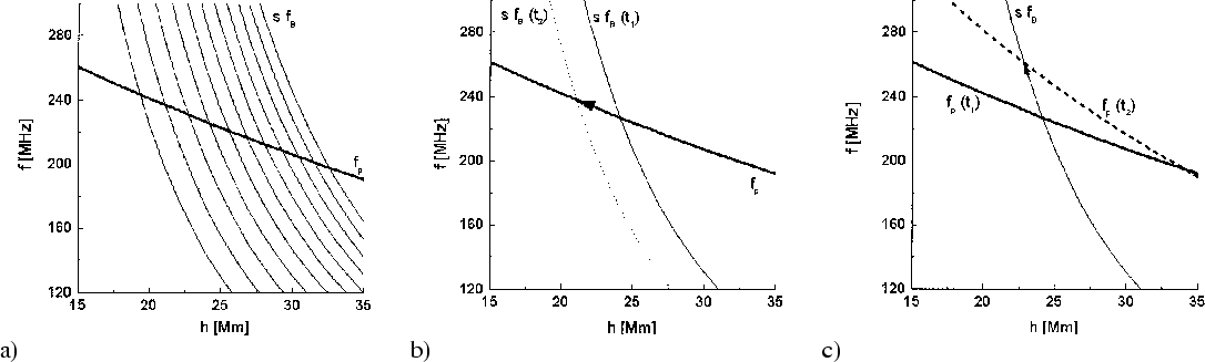 |
Figure 2:
The DPR source of ZP:
a) gyroharmonics sfB and plasma frequency |
| Open with DEXTER | |
The enhanced generation of electrostatic modes arises in the hybrid
band
![]() if the instability
occupies the wavelength interval with a normal dispersion law
(see Zheleznyakov & Zlotnik 1975). The highest increments appear near the
lower boundary of the hybrid band. The bandwidth of instability can be
much less that the distance fB between the harmonics for a sufficiently
high velocity of nonthermal electrons
if the instability
occupies the wavelength interval with a normal dispersion law
(see Zheleznyakov & Zlotnik 1975). The highest increments appear near the
lower boundary of the hybrid band. The bandwidth of instability can be
much less that the distance fB between the harmonics for a sufficiently
high velocity of nonthermal electrons![]() . The peak
increment doesn't markedly depend on the harmonic number. This is in
accordance with the observations.
. The peak
increment doesn't markedly depend on the harmonic number. This is in
accordance with the observations.
The consideration given in Appendices A and B refers to the instability
in the homogeneous plasma with constant electron density and
magnetic field. Now let us turn to a nonhomogeneous source
as shown in Fig. 1a. We assume that LS1 is filled
with equilibrium plasma (for the moment we do not invoke a possible influence
of the approaching flare ribbon) and a minor amount
of hot electrons with ring-type velocity distribution. If the gradients of
magnetic field and electron density along the lines of force are not the same,
the DPR condition (7) is realized at
discrete layers. These are defined
by the intersections of the curves
![]() and sfB in Fig. 2
and sfB in Fig. 2![]() . At these layers
the enhanced emission arises, and the dynamic spectrum will consist of
alternating dark and light stripes. It is easy to see that in the framework of
such a scheme the distance between the zebra stripes
. At these layers
the enhanced emission arises, and the dynamic spectrum will consist of
alternating dark and light stripes. It is easy to see that in the framework of
such a scheme the distance between the zebra stripes
The generation mechanism shown includes the nonlinear
transformation of longitudinal electrostatic waves-excited at the
upper hybrid frequency-into electromagnetic radiation freely
escaping the corona. The frequency interval between the stripes is
equal to (8) if the radiation is a result of the
coalescence of high frequency plasma waves (i.e. at a frequency
close to ![]() )
and some low frequency waves (for example,
whistlers or ion sound waves). Another transformation mechanism is
the scattering of plasma waves by ions. If the radio emission is a
result of the coalescence of two high frequency plasma waves, the
right side of (8) must increase by 2. Both cases can
be distinguished by polarization measurements. The radiation at
twice the plasma frequency should be only weakly polarized in a
relatively weak magnetic field. In our event the circular polarization
degree of ZP was -26%. Thus, the ZP are most
probably fundamental mode emission at the local plasma frequency.
The distance between the stripes is equal to (8). In
this paper we simply assume that the transformation took place
without further considering this necessary step to obtain
radio emission.
)
and some low frequency waves (for example,
whistlers or ion sound waves). Another transformation mechanism is
the scattering of plasma waves by ions. If the radio emission is a
result of the coalescence of two high frequency plasma waves, the
right side of (8) must increase by 2. Both cases can
be distinguished by polarization measurements. The radiation at
twice the plasma frequency should be only weakly polarized in a
relatively weak magnetic field. In our event the circular polarization
degree of ZP was -26%. Thus, the ZP are most
probably fundamental mode emission at the local plasma frequency.
The distance between the stripes is equal to (8). In
this paper we simply assume that the transformation took place
without further considering this necessary step to obtain
radio emission.
If for the characteristic length scales
![]() ,
then the distance
,
then the distance ![]() is equal to the electron gyrofrequency: this means
is equal to the electron gyrofrequency: this means
![]() .
In
this case we immediately find the magnetic field in the source. But if we apply
this approach to our data of interest, say at about 200 MHz with
.
In
this case we immediately find the magnetic field in the source. But if we apply
this approach to our data of interest, say at about 200 MHz with ![]() of
about 2 MHz, we obtain
of
about 2 MHz, we obtain ![]() .
If electrons
radiate at such high harmonics their energy must be rather great. Therefore the
weakly relativistic approximation is not valid. No zebra stripes
would appear.
.
If electrons
radiate at such high harmonics their energy must be rather great. Therefore the
weakly relativistic approximation is not valid. No zebra stripes
would appear.
Consequently, the inverse case must be more probable so that the magnetic field
changes with height faster than the electron density. This is the case in
Fig. 2. Here ![]() is LN/LB times less than the
gyrofrequency:
is LN/LB times less than the
gyrofrequency:
The described qualititative model of the source can easily
explain many features of ZP. It is seen from (9) and from
Fig. 2a that the frequencies at the DPR levels are not fully
equidistant. Moreover, in the framework of our source model
(under condition
![]() ), this distance increases with
frequency in accordance with observations. This can be nicely seen in Fig. 7 of
Paper I.
), this distance increases with
frequency in accordance with observations. This can be nicely seen in Fig. 7 of
Paper I.
Our source model can naturally explain the observed positive
frequency drift of zebra-stripes towards higher frequencies
when the burst decays. Such a drift is a common
feature for many ZP (see, for example, Slottje 1981). The positive
frequency drift can be caused by the decrease of the magnetic field in the
source: in this
case the set of curves sfB(h) in Fig. 2a is moving to
lower frequencies relative to the curve
![]() ,
and each point
of intersection - defining the frequency of a fixed stripe - is moving
up along the curve
,
and each point
of intersection - defining the frequency of a fixed stripe - is moving
up along the curve
![]() (Fig. 2b). The positive drift is
also obtained by a change of the steepness of the curve
(Fig. 2b). The positive drift is
also obtained by a change of the steepness of the curve
![]() :
if the scale
LN decreases with time towards the end of event (that means cooling of plasma
in the loop takes place), then the
curve
:
if the scale
LN decreases with time towards the end of event (that means cooling of plasma
in the loop takes place), then the
curve
![]() become steeper. The points of intersection with
harmonics sfB(h) are again moving up providing the positive frequency
drift of zebra stripes (Fig. 2c). An
increase of the distance between stripes with time seen on the dynamic spectrum
follows from the suggested scheme, too
become steeper. The points of intersection with
harmonics sfB(h) are again moving up providing the positive frequency
drift of zebra stripes (Fig. 2c). An
increase of the distance between stripes with time seen on the dynamic spectrum
follows from the suggested scheme, too![]() .
.
An essential feature of our source model is the spatial separation between sources of different stripes. From this point of view it might appear strange that the change of frequency of different stripes occurs synchronously. Actually, this is due to the fact that the collective processes prevail in the loop, and the magnetic trap changes as a whole. During the flare of interest, X-ray and radio data confirm a reformation of the field and density structure in the active region corona (Aurass et al. 1999).
From the previous discussion of the emission mechanism, the ZP gives
information
about magnetic fields in the corona. This is of some diagnostic importance
because direct measurements in the corona by optical observations are
impossible, and until now spatially resolved field estimates from radio data
were tried only using the well-known theory of microwave emission (e.g.
Gelfreikh 1998; Klein 1992).
However for AR NOAA 7792 the force-free extrapolated coronal field was derived
from photospheric field measurements (Paper I). In Fig. 3 we
present a typical height over field strength plot along a selected field line of
the FS loop system LS1 (compare Fig. 2 of Paper I).
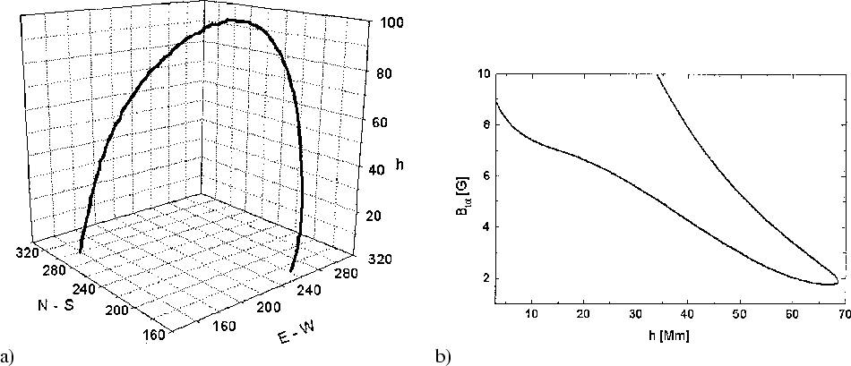 |
Figure 3: Magnetic field line selected from extrapolated LS1 (see Fig. 2 of Paper I): a) perspective view; b) height dependence of field strength. |
| Open with DEXTER | |
Thus, we can plot the dependence of gyrofrequency harmonics sfB(h) on the height and check for which density model the DPR effect appears. This must be compared with the zebra stripe frequencies (Fig. 4). Let us do this for certain selected times.
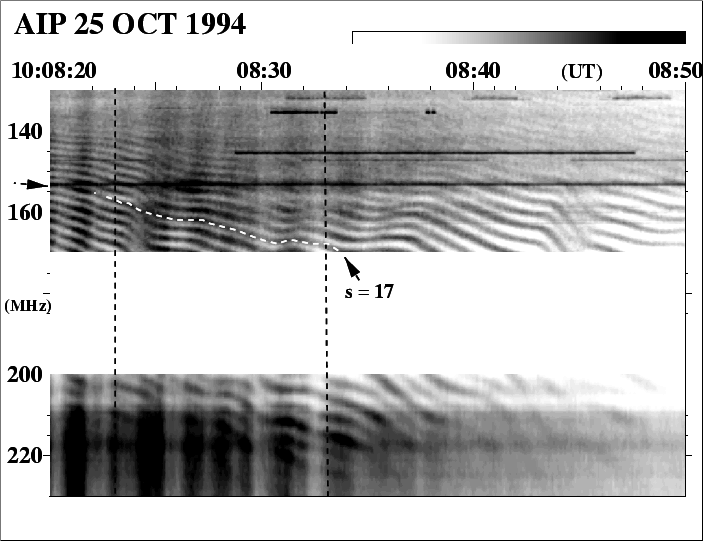 |
Figure 4:
The dynamic spectrum of ZP 10:08:
|
| Open with DEXTER | |
According to our scheme shown in Fig. 2a, the
minimum magnetic field at the loop apex corresponds to the maximum
harmonic number. The lowest frequency of ZP at 10:08:23 UT is
136.9 MHz (Fig. 4). The magnetic field along the chosen
line has its minimum value
![]() G at a height of
G at a height of
![]() km. We conclude that the highest harmonic number
at this moment is
km. We conclude that the highest harmonic number
at this moment is
![]() MHz
MHz
![]() .
Being bound to the height, we can determine the numbers of
harmonics of zebra stripes on the instantantaneous spectrum at
the moment 10:08:23 and plot dependencies sfB(h) for harmonics
.
Being bound to the height, we can determine the numbers of
harmonics of zebra stripes on the instantantaneous spectrum at
the moment 10:08:23 and plot dependencies sfB(h) for harmonics
![]() (Fig. 5a). Horizontal lines in this figure
are the observed frequencies on zebra stripes at the selected
moment. The points of intersection of two sets of curves (sfB
(h) and the observed frequencies of ZP) marked by dots are the
DPR levels. The line connecting these points is the
expected distribution of plasma frequency
(Fig. 5a). Horizontal lines in this figure
are the observed frequencies on zebra stripes at the selected
moment. The points of intersection of two sets of curves (sfB
(h) and the observed frequencies of ZP) marked by dots are the
DPR levels. The line connecting these points is the
expected distribution of plasma frequency
![]() (or electron
density) over the height.
(or electron
density) over the height.
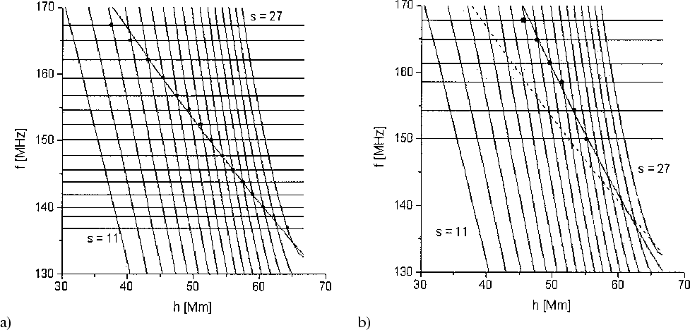 |
Figure 5:
Observations versus theory: horizontal lines are peak
frequencies of zebra stripes. A grid of gyroharmonics
|
| Open with DEXTER | |
To what extent does a distribution
correspond to the true electron density in the loop? The electron
density over height follows a barometric law because of
hydrostatic equilibrium (Priest 1987), so the plasma frequency
![]() decreases with the height in the following way:
decreases with the height in the following way:
Looking for the best fit
for matching two sets of frequencies (observed frequencies of
zebra stripes and the values given by intersection of the curves
![]() and sfB(h)) we found for the frequency interval
and sfB(h)) we found for the frequency interval
![]() MHz for the moment 10:08:23 UT:
MHz for the moment 10:08:23 UT:
![]() K
and
K
and
![]() MHz (
MHz (
![]() cm-3)
cm-3)![]() .
The dependence
.
The dependence
![]() is shown in Fig. 5a by a thick line.
The remaining intersection points are also situated at
the thick curve. This means that the frequencies of DPR levels given by the
theory coincide surprisingly well with observed frequencies of zebra stripes.
is shown in Fig. 5a by a thick line.
The remaining intersection points are also situated at
the thick curve. This means that the frequencies of DPR levels given by the
theory coincide surprisingly well with observed frequencies of zebra stripes.
It should be emphasized that we used two independent sets of data - the peak frequencies of zebra stripes and the extrapolated magnetic field along a field line - and obtained the electron density law. It was found to be a barometric distribution with a reasonable temperature. This fact is no coincidence. It undoubtedly confirms the DPR model of zebra stripe origin.
We will now use the same approach to calculate the observed stripes somewhat later. At 10:08:33 UT there was a maximum amount of harmonics at higher frequencies (Fig. 4). Let us assume that the magnetic field is the same as at 10:08:23 UT and try to understand what parameters are changed while the zebra stripes drifted to higher frequencies. Accepting the harmonic numbers for stripes at 10:08:23 UT we can follow the stripes and match the observed frequencies of stripes at 10:08:33 UT. For example, we followed the stripe s=17 (white dotted line on dynamic spectrum in Fig. 4).
This stripe corresponds to f=168 MHz on 10:08:33 UT.
Thus, having found the numbers of harmonics, we can get the expected DPR
points and plot Fig. 5b for the moment
10:08:33 UT. Here, we obtain a temperature of
![]() K (solid curve in Fig. 5b). For comparison, the curve
K (solid curve in Fig. 5b). For comparison, the curve
![]() for the moment 10:08:23 UT is shown in Fig. 5b by a dotted
line.
for the moment 10:08:23 UT is shown in Fig. 5b by a dotted
line.
The zebra stripe peak frequencies for both times reveal an increase of the exponent in the barometric electron density distribution and, consequently, a decrease of the plasma temperature within the 10 s interval between. Thus, if cooling of plasma in the trap happens in the way shown in Fig. 2c it can naturally explain the observed frequency drift of zebra stripes.
The relatively low temperature of the background plasma is not
surprising. As it is shown in Appendices A and B, the higher the
ratio
![]() ,
the better the conditions for the generation of
narrow band stripes at DPR levels (see Fig. A.1
with instability boundaries indicated). Calculations by Winglee
& Dulk (1986) confirmed the easier appearance of zebra stripes
at lower temperatures of the background plasma.
,
the better the conditions for the generation of
narrow band stripes at DPR levels (see Fig. A.1
with instability boundaries indicated). Calculations by Winglee
& Dulk (1986) confirmed the easier appearance of zebra stripes
at lower temperatures of the background plasma.
By matching of theoretical and observed
frequencies of zebra stripes we found a plasma temperature decrease
in the source volume with time. We
considered in the same manner as before the frequency spectrum at
10:08:48 UT when many stripes were
recorded. Again tracing a fixed harmonic from 10:08:23 UT
we find the numbers of harmonics at the later time. The temperature given by
fitting the barometric
distribution is now
![]() K. So, the ZP
time evolution gives convincing evidence of cooling of the
plasma in the coronal loop towards the end of the event.
K. So, the ZP
time evolution gives convincing evidence of cooling of the
plasma in the coronal loop towards the end of the event.
However, plasma cooling must not be the only reason for the
observed positive drift of zebra stripes. Bearing in mind that a fixed stripe
drifts to higher frequencies (the
harmonic s=17 is marked in Fig. 4), we can find from
the spectrum at 10:08:48 UT that the lowest frequency stripe
corresponds to a harmonic number s=32. This number requires
magnetic fields of
![]() G in the trap apex which is
less than the minimum magnetic field in our approximation derived
from the selected field line. We conclude that the magnetic field
decreases between 10:08:33 UT and 10:08:48 UT.
G in the trap apex which is
less than the minimum magnetic field in our approximation derived
from the selected field line. We conclude that the magnetic field
decreases between 10:08:33 UT and 10:08:48 UT.
Note that the decrease of the magnetic field will result in an apparent motion of the zebra stripe source to regions with greater electron density. This effect was observed in the radio images as a motion of the source with a velocity proportional to the drift rate of zebra stripes (Fig. 11 of Paper I).
By comparing the evolution of the stripe frequencies over time both effects - the plasma cooling and the decrease of the magnetic field - act in the same manner on the radiation pattern. With plasma temperature and magnetic field strength decay the stripes drift to higher frequencies and, simultaneously, more stripes become visible at the low frequency edge of the FS pattern. The rise of the emission frequency of a given stripe with time possibly reveals the temperature decay. The appearance of new stripes at the low frequency edge more probably may be interpreted as a decay of the reference field strength of stripe interpretation.
Note that in Fig. 5 we used only the assumption
that the lowest frequency of the ZP stripe at 10:08:23 UT corresponds to
the harmonic number s=27. In its turn this assumption is
based on the minimum magnetic field value
![]() G
at the top of LS1 along the selected field line. If we
admit that the ZP source extended not to the very top of the trap, and
the interval of harmonic numbers is, say,
G
at the top of LS1 along the selected field line. If we
admit that the ZP source extended not to the very top of the trap, and
the interval of harmonic numbers is, say,
![]() or
or ![]() ,
we can try to find the barometric
distribution corresponding to the DPR levels, but the fitting is much
worse than in Fig. 5a for
,
we can try to find the barometric
distribution corresponding to the DPR levels, but the fitting is much
worse than in Fig. 5a for
![]() .
For sets with lower
harmonic numbers, the line connecting the DPR levels cannot be reconciled with
any barometric distribution. Thus we claim that the height distributions of the
magnetic field and electron density shown in Fig. 5 are quite
reliable.
.
For sets with lower
harmonic numbers, the line connecting the DPR levels cannot be reconciled with
any barometric distribution. Thus we claim that the height distributions of the
magnetic field and electron density shown in Fig. 5 are quite
reliable.
We have considered above only one selected force line of the extrapolated magnetic field in the radio source loop LS1. It has been chosen because it is just in the center of the bunch of force lines of the magnetic field forming the shape of the coronal loop. The same procedure of fitting the DPR conditions for other field lines results in approximately the same harmonic numbers (with a small dispersion of the maximum s) and the parameters of the barometric distribution of the background plasma.
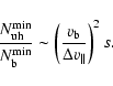
The strong ZP emission arises approximately 2.5 min after the BBP (see Paper I). Since the sources of BBP and ZP were located in the same coronal magnetic loop, this time delay implies that the ZP appearance was preceded by about 100 injections of fast particles into the magnetic trap. This is due to the fact that the instability threshold is markedly higher for plasma waves excited by the DPR effect than the threshold of beam instability which forms BBP.
Therefore, numerous injections of fast electron beams into the trap are necessary in order to "pump up'' a large number of energetic electrons and to "switch on'' the DPR instability. If injected beams are rather weak, then first the BBP appear, and after some time they can be accompanied by ZP.
When a fast electron beam is injected along the magnetic field of the trap
the increment of beam instability is determined by the relation:
Scattering of beam electrons on the excited plasma turbulence results in
an increase of
dispersion of fast electrons over the velocities perpendicular to the magnetic
field. Due
to the "loss cone'' in the trap, an anisotropic distribution function is formed
and special conditions are created for plasma
wave
generation in DPR regions. The highest increment of DPR instability at plasma
waves is
given by the relation (Zheleznyakov & Zlotnik 1975a):
Numerous injections
of electron beams into the coronal magnetic field result in
a gradual increase of trapped energetic particles and "switching on''
of the DPR instability. Therefore, the ZP shows a
tendency to appear at lower frequencies (
![]() MHz)
compared to pulsations (
MHz)
compared to pulsations (
![]() MHz). We believe the reason
is that the effective electron ion collision number restricting
the DPR instability threshold is lower near the trap apex than at
its footpoints. The amount of trapped particles tends to be
concentrated at the trap apex. So, the conditions for ZP generation
are better in the upper part of the coronal loop, this means at low observing
frequencies.
MHz). We believe the reason
is that the effective electron ion collision number restricting
the DPR instability threshold is lower near the trap apex than at
its footpoints. The amount of trapped particles tends to be
concentrated at the trap apex. So, the conditions for ZP generation
are better in the upper part of the coronal loop, this means at low observing
frequencies.
This paper gives a discussion of different theoretical approaches for the
physical understanding of some common solar radio type IV burst continuum fine
structures (FS). The FS of interest are broad band decimetric and metric radio
pulsations (BBP) with roughly persistent upper and lower frequency boundary in
the period range of ![]() s and special quasi-harmonic structure of the
spectrum known as a zebra pattern (ZP). In Paper I we presented an extended
discussion of a classic example of BBP and ZP thereby discussing the single FS element (the pulse and the zebra stripe) in spectral and radio imaging data.
Additionally we discussed a statistical analysis of the BBP period (for the
selected single event), the cross relationship between spatially split
sources of a single pulsation pulse, and a linear regression relation between
the local drift rate of a zebra stripe and the projected speed of zebra stripe
source motion in space. Based on Paper I we developed here (Paper II) a FS
source model. This model consists of an asymmetric loop configuration with an
electron accelerator at those footpoints where the magnetic flux is spatially
more concentrated. It turns out that the BBP periodicity follows from periodic
electron injections; it is an accelerator property. Further we understand that
ZP are due to distributed radio emission sources at double plasma resonance
levels near
the wider footpoint of the source model configuration. We demonstrate that the
observations of BBP and ZP can well be understood in the frame of our source
model. It allows us to decide between competing BBP and ZP mechanisms if we
specify those model parameters which we can obtain from the data set in Paper I.
s and special quasi-harmonic structure of the
spectrum known as a zebra pattern (ZP). In Paper I we presented an extended
discussion of a classic example of BBP and ZP thereby discussing the single FS element (the pulse and the zebra stripe) in spectral and radio imaging data.
Additionally we discussed a statistical analysis of the BBP period (for the
selected single event), the cross relationship between spatially split
sources of a single pulsation pulse, and a linear regression relation between
the local drift rate of a zebra stripe and the projected speed of zebra stripe
source motion in space. Based on Paper I we developed here (Paper II) a FS
source model. This model consists of an asymmetric loop configuration with an
electron accelerator at those footpoints where the magnetic flux is spatially
more concentrated. It turns out that the BBP periodicity follows from periodic
electron injections; it is an accelerator property. Further we understand that
ZP are due to distributed radio emission sources at double plasma resonance
levels near
the wider footpoint of the source model configuration. We demonstrate that the
observations of BBP and ZP can well be understood in the frame of our source
model. It allows us to decide between competing BBP and ZP mechanisms if we
specify those model parameters which we can obtain from the data set in Paper I.
We summarize and discuss in the following our results concerning the most probable BBP and ZP mechanisms.
We considered the distributions of magnetic field and electron density along the pulsation source volume and came to the conclusion that the Alfvén velocity inside the loop sharply increases from the loop apex to its footpoints. Therefore, MHD oscillations are not capable of inducing synchronous radio pulsations in a broad frequency band and we can exclude them from the BBP mechanisms.
The BBP source was moving yielding a negative frequency drift typical of type III and J bursts. The direction of the motion coincided approximately with the projection of the trap axis on the photosphere. This fact, together with the wide source branching at the high frequency edge of the discussed BBP (Paper I) favours assuming that the BBP were driven by a periodic injection of fast electron beams into the coronal magnetic field. This generation mechanism is similar to that of type III bursts.
The source of fast electrons was located in one of the footpoints of the loop which was embedded in the strong magnetic field of a north polarity sunspot. Near this sunspot, emerging magnetic flux of opposite polarity was observed. We suppose that this emerging flux was connected with a current-carrying magnetic loop (EL in Fig. 1), which interacted with the large coronal magnetic loop LS1. We discussed two possible mechanisms of pulsating particle acceleration - pulsed dynamics of explosive magnetic reconnection when two magnetic loops LS1 and EL collide (Tajima et al. 1987), and acceleration by an electrostatic field in the compact current-carrying loop EL. If we consider the loop EL as an equivalent circuit, the modulation of acceleration occurs due to RLC oscillations (Zaitsev et al. 1998). The pulsed regime of explosive reconnection cannot explain BBP in the event of interest because this effect can provide only a few pulsation pulses (Tajima et al. 1987).
The origin of ZP is
enhanced generation of plasma waves in regions of
inhomogeneous coronal magnetic traps where the condition of double
plasma resonance
![]() is fulfilled (DPR levels). We checked this by
deriving the
(unknown) coronal gyrofrequency from the
force-free extrapolated magnetic field together with the radio source site
information. The height dependence of the density was found to be well in
accordance with a
barometric density law assuming
is fulfilled (DPR levels). We checked this by
deriving the
(unknown) coronal gyrofrequency from the
force-free extrapolated magnetic field together with the radio source site
information. The height dependence of the density was found to be well in
accordance with a
barometric density law assuming
![]() K.
We obtained a good coincidence between
the stripe frequencies predicted by theory and the observed stripe pattern.
The observed increase of intervals between stripes with frequency and time
is also well confirmed by the theory.
K.
We obtained a good coincidence between
the stripe frequencies predicted by theory and the observed stripe pattern.
The observed increase of intervals between stripes with frequency and time
is also well confirmed by the theory.
The considered zebra stripes show a positive frequency drift of up to
2 MHz s-1. In the framework of the DPR
mechanism this follows from plasma cooling in the trap
(that results in the increase of the electron density gradient and a shift
of the points of intersection of the curves sfB(h) and
![]() towards higher frequencies) or/and by expansion of the loop LS1
(that results in a decrease of magnetic field).
The same effects can explain the downward motion of the ZP source.
The DPR instability has a much higher threshold value of fast electron
density than the beam instability. This explains the time delay
between BBP and ZP.
towards higher frequencies) or/and by expansion of the loop LS1
(that results in a decrease of magnetic field).
The same effects can explain the downward motion of the ZP source.
The DPR instability has a much higher threshold value of fast electron
density than the beam instability. This explains the time delay
between BBP and ZP.
We have shown that the dynamic spectrum of ZP in the event of interest with relatively large numbers of radiation stripes cannot be understood by excited Bernstein modes. We can also exclude nonlinear scattering of plasma waves on whistlers (Chernov 1976, 1990): it is unlikely that solitary whistler waves are positioned in an inhomogeneous coronal magnetic loop just according to a definite law in order to provide the systematic increase of the interval between the stripes with frequency.
The main results of our case study of type IV radio burst fine structures - broad band pulsations (BBP) and zebra patterns (ZP) - can be summarized as:
Acknowledgements
We are grateful to K.-L. Klein for his cooperation in Part I of this work. The present work was possible due to joint grants 02-02-04005 (RFBR-DFG) and 436RUS 113/675/2-1 R (DFG-RFBR). The authors are grateful to the Deutsche Forschungsgemeinschaft and the Russian Foundation for Basic Research. The work by E.Z. and V.Z. was also supported by RFBR grants 01-02-17252 and 02-02-16239. The authors are thankful to the referee, Dr. Jan Kuijpers, for useful comments.
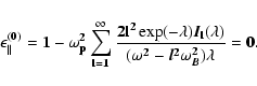
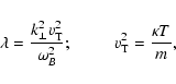
We emphasize some aspects of the theory of longitudinal wave
excitation by trapped electrons considering only the kinetic instability. The
hydrodynamic instability requires much higher values of nonequilibrium electron
densities.
We assume that the density of nonequilibrium electrons is small
compared to background plasma. The dispersion properties of the
waves are determined by the equilibrium component and can be described by
well-known equations (for example Bekefi 1971; Zheleznyakov
1977, 2000):
Note that the behaviour of the dispersion curves as shown in
Fig. A.1 for longitudinal waves in the vicinity of
the hybrid frequency remains only under the condition
![]() .
Its violation results in
strong damping of electrostatic modes in the background plasma. If
the angle between the wave vector
.
Its violation results in
strong damping of electrostatic modes in the background plasma. If
the angle between the wave vector ![]() and the magnetic field
and the magnetic field
![]() is far enough from
is far enough from ![]() (
(
![]() )
the solutions of the dispersion equation are close to
the well known expressions for the isotropic plasma under the
condition
)
the solutions of the dispersion equation are close to
the well known expressions for the isotropic plasma under the
condition
![]() (for example Ginzburg 1967;
Zheleznyakov 2000; Melrose 1980).
(for example Ginzburg 1967;
Zheleznyakov 2000; Melrose 1980).
Following Zheleznyakov & Zlotnik (1975)![]() and Winglee & Dulk (1986),
we will consider the distribution function of nonequilibrium
electrons in the form
and Winglee & Dulk (1986),
we will consider the distribution function of nonequilibrium
electrons in the form
It is important that the
![]() -dependence of
-dependence of ![]() (B.3) is due to the function
(B.3) is due to the function
![]() .
Hence for a fixed frequency and the corresponding values
.
Hence for a fixed frequency and the corresponding values
![]() the increment is peaked at
the increment is peaked at
![]() ,
that is at an optimal value:
,
that is at an optimal value:
It should be noted that all formulas after (B.7)
are valid only if
![]() .
They are
given to show the qualititative behaviour of the growth
rate and to outline the boundary parameters.
.
They are
given to show the qualititative behaviour of the growth
rate and to outline the boundary parameters.
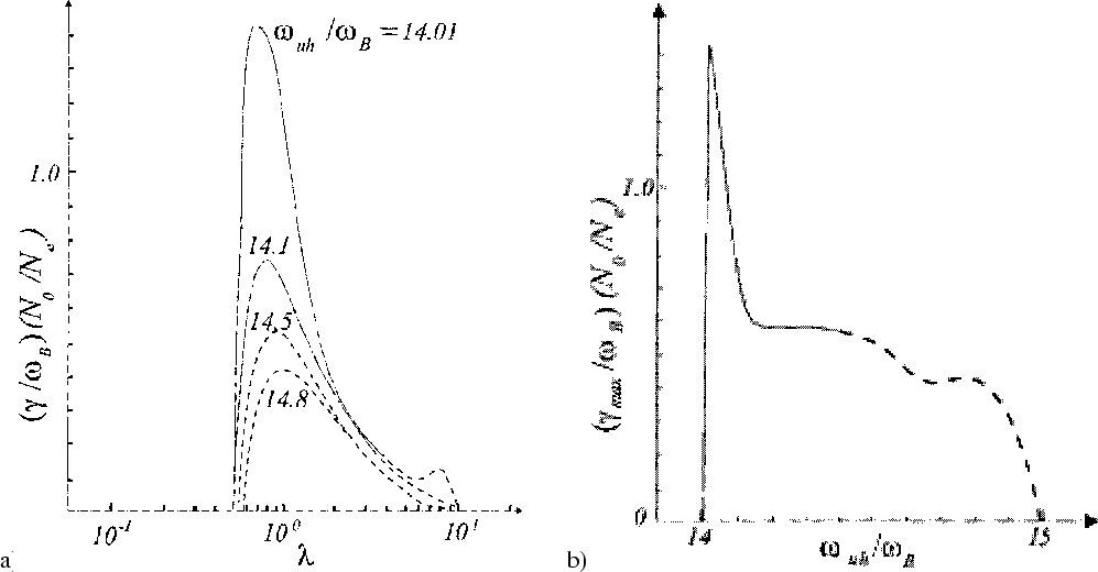 |
Figure B.1:
The growth rate of the waves in the hybrid band
|
Note that the hybrid band is not distinguished by values of
![]() against other harmonic bands:
the numerator in the growth rate
against other harmonic bands:
the numerator in the growth rate ![]() (B.3) (including
the position of instability boundaries) behaves similar for
Bernstein modes and for waves in the hybrid band. The dispersion
curves at
(B.3) (including
the position of instability boundaries) behaves similar for
Bernstein modes and for waves in the hybrid band. The dispersion
curves at
![]() drastically distinguish the hybrid band from other harmonic
intervals. Instead of anomalous dispersion typical for Bernstein
modes at
drastically distinguish the hybrid band from other harmonic
intervals. Instead of anomalous dispersion typical for Bernstein
modes at
![]() ,
the normal dispersion described
approximately by (A.6) takes place. A specific feature
of such dispersion is that the derivative
,
the normal dispersion described
approximately by (A.6) takes place. A specific feature
of such dispersion is that the derivative
![]() is considerably
less than that of Bernstein modes and for branches of dispersion
curves with anomalous dispersion in the hybrid band at
is considerably
less than that of Bernstein modes and for branches of dispersion
curves with anomalous dispersion in the hybrid band at
![]() .
.
A strong instability is realized at
sufficiently great velocities ![]() of the nonequilibrium
electrons (
of the nonequilibrium
electrons (
![]() )
when the instability boundary
)
when the instability boundary
![]() is located in the region of the
normal dispersion (
is located in the region of the
normal dispersion (
![]() ).
Taking into account (B.11) and the fact that the dispersion
in the hybrid band changes its sign at
).
Taking into account (B.11) and the fact that the dispersion
in the hybrid band changes its sign at
![]() ,
we conclude that
the enhanced radiation at
,
we conclude that
the enhanced radiation at
![]() (the DPR effect) can occur under the
condition:
(the DPR effect) can occur under the
condition:
The peak increment weakly depends on the harmonic number
s if the conditions (B.8)-(B.12) are valid. Actually it is
mainly determined by the minimum of the function
![]() which doesn't change markedly with index s.
which doesn't change markedly with index s.
It should be also noted that at high harmonics the
frequency intervals where the relativistic effects
have to be taken into account can occupy a marked part of the hybrid band.
In the frequency interval
We obtain the following peak growth rate for
![]() and
the ratio
and
the ratio
![]() .
.
In order to estimate the frequency interval in which the enhanced
generation takes place, we refer to the relations (B.5),
(B.6) and (A.6). A typical scale of change of
the function
![]() ,
determining the growth rate, is
,
determining the growth rate, is
![]() ,
i.e.
,
i.e.
The dependence of the maximum growth rate (over all ![]() )
on
the ratio
)
on
the ratio
![]() (that is, on the position of the
upper hybrid frequency inside the hybrid band) shown in Fig. B.1b
is explained as follows. If
(that is, on the position of the
upper hybrid frequency inside the hybrid band) shown in Fig. B.1b
is explained as follows. If
![]() is far from
is far from
![]() and
and
![]() ,
in the region of the normal
dispersion the derivative in the denominator in (B.3)
varies only slightly with
,
in the region of the normal
dispersion the derivative in the denominator in (B.3)
varies only slightly with
![]() (at great s). When
(at great s). When
![]() approaches the lower boundary of the hybrid band
approaches the lower boundary of the hybrid band
![]() ,
the growth rate increases due to the multiplier
,
the growth rate increases due to the multiplier
![]() in
in
![]() ,
written similarly to (B.7) for the harmonic s-1.At
the upper boundary of the hybrid band (
,
written similarly to (B.7) for the harmonic s-1.At
the upper boundary of the hybrid band (
![]() )
the growth rate doesn't increase or increases only
slightly since in the interval
)
the growth rate doesn't increase or increases only
slightly since in the interval
![]() the non-relativistic approximation for
the non-relativistic approximation for
![]() (B.10) breaks and the value zs in (B.7)
markedly decreases. When
(B.10) breaks and the value zs in (B.7)
markedly decreases. When
![]() is close to
is close to
![]() or
or
![]() ,
the dispersion curves approach the
harmonics. Then in the expression for
,
the dispersion curves approach the
harmonics. Then in the expression for
![]() (A.4) the resonance term involving the multiplier
(A.4) the resonance term involving the multiplier
![]() or
or
![]() dominates. As a result, the value
dominates. As a result, the value
![]() increases sharply, leading to the decrease of the growth
rate in a small region around points
increases sharply, leading to the decrease of the growth
rate in a small region around points
![]() and
and
![]() .
.
![\begin{displaymath}\dot N [{\mbox s}^{-1}]=0.35 N\nu_{\rm ei} V
\left(\frac{E_{\...
...}} {E_{\parallel}}} -
\frac{E_{\rm D}}{4E_{\parallel}}\right],
\end{displaymath}](/articles/aa/full/2003/42/aa4049/img97.gif)


![\begin{displaymath}\omega^2-s^2\omega_B^2 =
\frac{\omega_{\rm p}^2\omega_B^2}{[(...
...^2]}
\frac{s(s+1)}{(s-2)!}\left(\frac{\lambda}{2}\right)^{s-1}
\end{displaymath}](/articles/aa/full/2003/42/aa4049/img197.gif)


![\begin{displaymath}\gamma={\mbox{Im}}\omega\approx -\frac{Im
\epsilon_{\parallel...
...}/\partial\omega
\right]}_{\epsilon_{\parallel}^{(0)}=0}}\cdot
\end{displaymath}](/articles/aa/full/2003/42/aa4049/img230.gif)
![\begin{displaymath}\mbox{Im}\epsilon_{\parallel}^{(1)}=\sqrt{\frac{\pi}{2}}
\fra...
...}\left[\delta_l\varphi_l +(\delta_l+1)\zeta\varphi'_l
\right],
\end{displaymath}](/articles/aa/full/2003/42/aa4049/img236.gif)