

One of the major goals of our observations of GD 358 was to discover additional modes to help refine our seismological model fits. We were also interested in how much the globally optimal model parameters would change due to the slight shifts in the observed periods. With these goals in mind, we repeated the global model-fitting procedure of Metcalfe, Winget & Charbonneau (2001) on several subsets of the new observations.
Our model-fitting method uses the parallel genetic algorithm described by
Metcalfe & Charbonneau (2003) to minimize the root-mean-square (rms)
differences between the observed and calculated periods (Pk) and
period spacings (
 )
for models with effective
temperatures (
)
for models with effective
temperatures (
 )
between 20 000 and 30 000 K, total stellar
masses (M*) between 0.45 and 0.95
)
between 20 000 and 30 000 K, total stellar
masses (M*) between 0.45 and 0.95  ,
helium
layer masses with
,
helium
layer masses with
 between 2.0 and
  7.0, and an internal C/O
profile with a constant oxygen mass fraction (
7.0, and an internal C/O
profile with a constant oxygen mass fraction ( )
out to some
fractional mass (q) where it then decreases linearly in mass to zero
oxygen at
0.95 m/M*. This technique has been shown to find the globally
optimal set of parameters consistently among the many possible
combinations in the search space, but it requires between 200 and
4000 times fewer model evaluations than an exhaustive search of the
parameter-space to accomplish this, and has a failure rate <10-5.
)
out to some
fractional mass (q) where it then decreases linearly in mass to zero
oxygen at
0.95 m/M*. This technique has been shown to find the globally
optimal set of parameters consistently among the many possible
combinations in the search space, but it requires between 200 and
4000 times fewer model evaluations than an exhaustive search of the
parameter-space to accomplish this, and has a failure rate <10-5.
We attempted to fit the 13 periods and period spacings defined by the
m=0 components of the 14 modes identified as k=7 to k=20 in
Table 9. Because of our uncertainty about the proper
identification of
k=18(see Sect. 4) we performed fits under two different assumptions: for Fit
a we assumed that the frequency near 1233  Hz was k=18 (similar to
the frequency identified in 1990), and for Fit b we assumed that the
larger amplitude frequency near 1255 Hz was k=18. The results of
these two fits led us to prefer the identification for k=18 in Fit a,
and we included this in an additional fit using only the 11 modes from
k=8 to k=18, which correspond to those identified in 1990 (Fit c).
We performed an additional fit (Fit d) that included the same 13 periods
used for Fit a, but ignored the period spacings.
The optimal values for the five model parameters, and the root-mean-square
residuals between the observed and computed periods (
Hz was k=18 (similar to
the frequency identified in 1990), and for Fit b we assumed that the
larger amplitude frequency near 1255 Hz was k=18. The results of
these two fits led us to prefer the identification for k=18 in Fit a,
and we included this in an additional fit using only the 11 modes from
k=8 to k=18, which correspond to those identified in 1990 (Fit c).
We performed an additional fit (Fit d) that included the same 13 periods
used for Fit a, but ignored the period spacings.
The optimal values for the five model parameters, and the root-mean-square
residuals between the observed and computed periods ( )
and
period spacings (
)
and
period spacings (
 )
for the four fits are shown in
Table 10.
)
for the four fits are shown in
Table 10.
| Parameter | Fit a | Fit b | Fit c | Fit d |
 |
24 300 | 23 500 | 24 500 | 22 700 |
 |
0.61 | 0.60 | 0.625 | 0.630 |
 |
-2.79 | -5.13 | -2.58 | -4.07 |
|
0.81 | 0.99 | 0.39 | 0.37 |
| q (m/M*) | 0.47 | 0.47 | 0.83 | 0.42 |
 |
2.60 | 3.65 | 2.12 | 1.72 |
 |
4.07 | 4.92 | 2.21 |  |
Our preferred solution from Table 10 is Fit a, because it
includes our favored identification for the k=18 mode and the additional
pulsation periods. The larger
in Fit a compared to
Fit c is dominated by the large period spacings between the k=19 and
20 modes (47.6 s) and the k=7 and 8 modes (49.4 s). Fit a has a
mass and effective temperature that are essentially the same as the fit of
Bradley & Winget (1994), and are consistent with the spectroscopic
values derived by Beauchamp et al. (1999). The other structural parameters
are otherwise similar to those found by Metcalfe et al. (2001)
(
 K,
K,
 ,
,
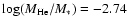 ,
,
 ,
and q = 0.49). We caution, however, that the large
values of
and
for Fit a imply that our
model may not be an adequate representation of the real white dwarf star.
New and unmodeled physical circumstances may have arisen between 1994 and
2000 (e.g. whatever caused the forte in 1996), which may account for
the diminished capacity of our simple model to match the observed periods.
,
and q = 0.49). We caution, however, that the large
values of
and
for Fit a imply that our
model may not be an adequate representation of the real white dwarf star.
New and unmodeled physical circumstances may have arisen between 1994 and
2000 (e.g. whatever caused the forte in 1996), which may account for
the diminished capacity of our simple model to match the observed periods.
Copyright ESO 2003