4 Chamaeleon I

Our main source of data regarding the Chamaeleon I association is the work by Lawson et al. (1996): we use their member list (117 stars in their Table B1) and their estimates of $L_{\rm bol}$ and $T_{\rm eff}$ (available for 78 stars, Table 6). We adopt here a distance to the Chamaeleon I cloud of 160 pc (Whittet et al. 1997; Wichmann et al. 1998), 20 pc larger than the distance assumed by Lawson et al. (1996) in estimating bolometric luminosities. We therefore increased the $L_{\rm bol}$ values accordingly. Masses of 71 candidate members were derived from placement in the HR diagram and interpolation of Siess et al. (2000) evolutionary tracks.

The selection of candidate members in Lawson et al. (1996) is performed mainly on the basis of either their H $_{\rm\alpha }$ or X-ray emission. The danger of preferentially selecting faint stars (both optically and in X-rays) with strong H $_{\rm\alpha }$ emission is therefore present. However the Chamaeleon I association is close enough that a large fraction of intermediate mass members is probably detected in the ROSAT PSPC X-ray observations. Also, as anticipated in the introduction, other than $L_{\rm X}$ we will also investigate the dependence of $L_{\rm X}/L_{\rm bol}$ on circumstellar characteristics and, as a further test, we will also consider a fully X-ray selected sample.

X-ray data were taken from Lawson et al. (1996): they quote X-ray luminosities (or upper limits) for members of the region, computed from ROSAT PSPC count rates in the 0.4-2.5 keV spectral band (Feigelson et al. 1993), using a constant count-rate to $L_{\rm X}$ (in the same band) conversion factor: 1 PSPC count $\rm ks^{-1}=3\times10^{28}~ \rm ergs \ s^{-1}$. Feigelson et al. (1993) find that this conversion factor corresponds to assuming a plasma temperature $kT \sim 1$ keV and an absorption by a hydrogen column, $N_{\rm H}$, corresponding to $A_{V} \sim 1$.

In order to account for differential extinction (i.e. the fact that star are subject to different extinctions) and to uniform our assumptions to the ONC and NGC 2264 studies, we re-estimated X-ray luminosities, in our standard 0.1-4.0 keV band. We started from PSPC count rates in the 0.4-2.5 keV band, i.e. from the $L_{\rm X}$ reported in Lawson et al. (1996) divided by the above mentioned conversion factor. We then multiplied these count-rates by conversion factors between PSPC count-rates (in the 0.4-2.5 keV band) and luminosities (in the 0.1-4.0 keV band), computed for a kT=2.16 keV thermal plasma emission absorbed by an hydrogen column $N_{\rm H}=2 \times 10^{21}\cdot A_{V}$ and our assumed distance to the association (160 pc). Estimates of individual optical extinction values are taken from the following works: Lawson et al. (1996, A_J, Table 3), Gauvin & Strom (1992, A_V, Table 2), Walter (1992, E_B-V, Table 1) and Cambresy et al. (1998, A_V, Table 1); whenever multiple estimates were available for a given star we choose one of the four values, the precedence order being the same as the order of citation given above. A_J and E_B-V were converted to A_V by multiplying by 3.55 and 3.1 respectively (Mathis 1990). Figure 7 compares the new X-ray luminosities with those reported in Lawson et al. (1996) and indicates the effects that contribute to the considerable average discrepancy between the two estimates. First of all a difference of ${\sim} 0.15$ dex, indicated by the lowest diagonal thin line, is of unclear origin: we recomputed the conversion factor, in the 0.4-2.5 keV band, assuming kT=1.0 keV and $N_{\rm H}=2.0\times 10^{21}$, i.e. following Feigelson et al. (1993), and derived a larger conversion factor, by ${\sim} 0.15$ dex, respect to the value reported by these authors. The other light lines show the effect of having changed the assumed cluster distance, the chosen spectral band, the plasma temperature, and the average source extinction. The combined effects of these changes results in our X-ray luminosities being on average ${\sim} 5$ (0.7 dex) times larger than the ones formerly derived.

Figure 7: Comparison of X-ray luminosities reported by Lawson et al. (1996) for Chamaeleon I stars and those recomputed from the same data in this work. No distinction is made here between detections and upper limits. The bottom solid line indicates the locus of equal values; the light lines indicate the effect, on the X-ray luminosities, of: recomputing the conversion factor assuming kT=1.0 and $N_{\rm H}=2\times 10^{21}$ (see text), changing the assumed distance, source plasma temperature, band in which $L_{\rm X}$ is computed and average extinction. The scatter of points about the highest light line is due to the adoption of individual extinction corrections.

4.1 Activity vs. circumstellar environment

We adopt the distinction between CTTS and WTTS presented by Lawson et al. (1996, Table B1), excluding from our analysis 4 stars with uncertain classification, out of our 71 with mass estimates. The distinction is based on H $_{\rm\alpha }$emission. Our final sample comprises 28 CTTS and 39 WTTS.

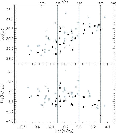Figure 8: $L_{\rm X}$ and $L_{\rm X}/L_{\rm bol}$ vs. mass for CTTS and WTTS (black and and gray symbols, respectively) belonging to the Chamaeleon I region. Filled circles represent detections, down-pointing arrows upper-limits.

Figure 8 shows, with different symbols for CTTS and WTTS, the scatter plots of $L_{\rm X}$ and $L_{\rm X}/L_{\rm bol}$ with mass. Disregarding for the moment the difference between CTTS and WTTS, a trend of increasing $L_{\rm X}$ with increasing mass, already noted by Lawson et al. (1996) and also seen in other star forming regions, can be clearly observed. $L_{\rm X}/L_{\rm bol}$ seems to be close to the saturation level (10^-3) at all masses. We note that Lawson et al. (1996), on the basis of their lower X-ray luminosities had excluded that coronal activity in Chamaeleon I members was saturated, contrary to what reported for other star forming regions. Our re-analysis of the same data shows that this result can be attributed in large part to the assumptions made in the conversion between count-rates and X-ray luminosities and to the choice a non standard X-ray spectral band for the calculation of $L_{\rm X}$.

Figure 9: Distributions of $L_{\rm X}$ and $L_{\rm X}/L_{\rm bol}$ (left and right columns) for CTTS and WTTS (solid and dashed lines, respectively) in the Chamaeleon I region. Each panel refers to a different mass range as indicated. Legends inside panels as in Fig. 2.

Figure 9 shows the $L_{\rm X}$ and $L_{\rm X}/L_{\rm bol}$ distribution functions, separately for CTTS and WTTS, in the same two mass ranges investigated in NGC 2264 and for the whole sample. First of all we note that there is little difference (at the ${\sim} 1\sigma$ level) between the two XLFs referring to the whole population. This is indeed the same result reported by Lawson et al. (1996). However a look at Fig. 8 shows that this might be due to the inclusion of stars over an ample range of masses. If we indeed consider only stars in the $0.5{-}1.0~M_\odot$ range CTTS appear to be underluminous respect to WTTS at the ${\sim} 3\sigma$ level, both in absolute terms and respect to their bolometric luminosities. $L_{\rm X}/L_{\rm bol}$ is indeed lower (at the $2{-}2.8\sigma$ level) even if we consider the whole sample. We obtain similar results, although of somewhat lesser significance, if we only consider X-ray selected stars: for example, the significance of the difference in the $0.5{-}1.0~M_\odot$ range are ${\sim} 1.5$ and ${\sim} 2.0\sigma$ for $L_{\rm X}$ and $L_{\rm X}/L_{\rm bol}$, respectively.

As a final note we remark that less significant results are obtained if the same analysis is performed with the values of $L_{\rm X}$ reported by Lawson et al. (1996). The scatter of points around the mean relations observed in Fig. 8, as well as in the distribution functions in Fig. 9, appear in this case to be larger. However the difference in the $0.5{-}1.0~M_\odot$ mass range remains (at the 2.2/2.8$\sigma$ level).