5 Discussion

Only a few active stars investigated until now have shown clear rotational modulation of line-depth ratios (e.g. $\sigma~$Dra, Gray et al. 1992; $\xi~$Boo A, Toner & Gray 1988). However all these studies have been devoted to young main-sequence stars with an activity degree detectably lower than RS CVn and BY Dra binaries and, consequently, with a temperature variation of only a few degrees or a bit more. Conversely, many more cases of long-term variation of average temperature have been found and have been attributed to stellar activity cycles similar to the 11-year solar one (e.g. Gray et al. 1996a, 1996b). These detections have been possible thanks to the large number of spectra collected in each season and averaged together with a great improvement of the S/N ratio.

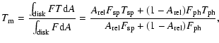
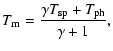
Since the temperature curves we obtained are $T_{\rm eff}$ averaged over the visible hemisphere, it is not possible to deduce directly the value of the spot temperature because the effect of the filling factor influences also this diagnostic. The dependence of average temperature on the spot relative area is different that of light curves. We can express the hemisphere-averaged temperature as

 

$$T_{\rm m} = \frac{\int\displaylimits_{{\rm disk}} F T {\rm d}A}{\... ... F_{\rm ph} T_{\rm ph}}{A_{\rm rel} F_{\rm sp} + (1 - A_{\rm rel}) F_{\rm ph}},$$ (11)

where $A_{\rm rel}$ is the projected area of the spot (or spots) relative to the stellar disk, $T_{\rm sp}$ and $T_{\rm ph}$ are the temperatures of spot and quiet photosphere, respectively, and $F_{\rm sp}$ and $F_{\rm ph}$ are the fluxes emitted per unit area by the spot and the photosphere at the continuum of observation wavelength, respectively.

Equation (11) can be also written as

 

$$T_{\rm m} = \frac{\gamma T_{\rm sp} + T_{\rm ph}}{\gamma + 1},$$ (12)

where $\gamma = \frac{A_{\rm rel}}{1 - A_{\rm rel}} \frac{F_{\rm sp}}{F_{\rm ph}}$.

If the spot is very cool, its contribution to the mean temperature is negligible because the flux ratio $\frac{F_{\rm sp}}{F_{\rm ph}}$ goes very rapidly to zero (much faster than $\frac{T_{\rm sp}}{T_{\rm ph}}$) with the decrease of $T_{\rm sp}$. Then $\gamma$ tends to zero and the average temperature tends to equal the photospheric one, so that a very large spot area would be required to account for the observed temperature variation.

In the opposite case, when $\frac{T_{\rm sp}}{T_{\rm ph}}$ approaches unity, the average temperature $T_{\rm m}$ is not appreciably changed by the passage of spots over the visible hemisphere. Again, very large spots are needed to reproduce the observed $T_{\rm m}$ variation. Then, there is a limited range for physically reliable solutions. In particular, given an observed variation amplitude $\Delta T_{\rm eff}$, there is a minimum spot area that can reproduce the observations.

As a first approximation we can estimate this minimum spotted area assuming that it is concentrated in only one hemisphere, and its passage causes the observed temperature decrease $\Delta T_{\rm eff}$. The maximum temperature value is assumed as the effective unspotted temperature ( $T_{\rm ph}$) of the star.

Starting from relation 12, we have numerically searched in the $\frac{T_{\rm sp}}{T_{\rm ph}}$- $A_{\rm rel}$ plane the solution for the minimum $A_{\rm rel}$ value compatible with the observed $\Delta T_{\rm eff}$ for each program star. The flux ratio $\frac{F_{\rm sp}}{F_{\rm ph}}$ has been evaluated as the ratio of the Planck functions at the average wavelength of observations, $\frac{B(\lambda,T_{\rm sp})}{B(\lambda,T_{\rm ph})}$.

We have no information on the maximum magnitude at the time of observation with respect to the unspotted magnitude of our program stars, however, we would like to remark that the maximum values of temperature we determined for all the three active stars are in very good agreement with the effective temperature reported in the literature. This proves the power of LDRs as temperature indicators as already pointed out by previous works (Gray 1989; Gray & Johanson 1991). The largest uncertainty in this task, as stressed by Gray (1989), is given by the setting of the absolute scale of temperature for a set of standard stars, while it is differentially possible to put in a growing temperature order each observed star with a precision of about 10 K, which amounts to about one hundredth of spectral subclass or 0.004 mag on B-V color index (Gray 1989; Gray & Johanson 1991).

Figure 14 displays the solutions in the plane $\frac{T_{\rm sp}}{T_{\rm ph}}$- $A_{\rm rel}$ for VY Ari with $T_{\rm ph}$ = 4916 K and $\Delta T_{\rm eff}=$ 177 K. The plot shows the parabolic shape of the family of solutions, which has a minimum fractional area 41% of the projected disk (corresponding to a radius of 40$^{\circ}$ for a single circular spot passing at the disk center) for a temperature ratio of 0.82. This constitutes a lower limit for the spot filling factor, and an average temperature for the spotted area $T_{\rm sp}$ = 4030 K.

Figure 14: Solutions of VY Ari $T_{\rm eff}$ curve for different spots temperature $\frac{T_{\rm sp}}{T_{\rm ph}}$. A lower limit for the fractional area $A_{\rm rel}$ of about 41% for $\frac{T_{\rm sp}}{T_{\rm ph}}~\simeq~0.82$ is apparent.

The solutions in the plane $\frac{T_{\rm sp}}{T_{\rm ph}}$- $A_{\rm rel}$ for IM Peg are shown in Fig. 15. A lower limit for the projected fractional area $A_{\rm rel}$ of $\simeq$32% (corresponding to a radius of 34$^{\circ}$ for a single circular spot passing at the disk center) is found for a temperature ratio of about 0.84. Given a maximum temperature $T_{\rm ph}$ = 4666 K, we obtain a spot temperature $T_{\rm sp}$ = 3920 K.

Figure 15: Solutions of IM Peg $T_{\rm eff}$ curve for different spots temperature $\frac{T_{\rm sp}}{T_{\rm ph}}$. A lower limit for the fractional area $A_{\rm rel}$ of about 32% for $\frac{T_{\rm sp}}{T_{\rm ph}}~\simeq~0.84$ is apparent.

The solutions in the plane $\frac{T_{\rm sp}}{T_{\rm ph}}$- $A_{\rm rel}$ for HK Lac are shown in Fig. 16. The minimum projected fractional area 34% (corresponding to a radius of 35$^{\circ}$ for a single circular spot passing at the disk center) is obtained for a temperature ratio of about 0.83. The assumed temperature maximum is $T_{\rm ph}$ = 4765 K, and the corresponding spot temperature is $T_{\rm sp}$ = 3955 K.

Figure 16: Solutions of HK Lac $T_{\rm eff}$ curve for different spots temperature $\frac{T_{\rm sp}}{T_{\rm ph}}$. A lower limit for the fractional area $A_{\rm rel}$ of about 34% for $\frac{T_{\rm sp}}{T_{\rm ph}}~\simeq~0.83$ is apparent.

If the maximum temperature does not really represent the unspotted photospheric temperature, we would be underestimating the spots area at each fixed $\frac{T_{\rm sp}}{T_{\rm ph}}$. In any case, we are considering the area of unevenly distributed spots, i.e. those giving rise to the observed modulation. We cannot argue, on the basis of only one temperature maximum value, the presence of a contribution from additional evenly distributed spot groups, like for example an equatorial spot belt or a large polar spot, because we would have information about the "unspotted temperature"; likewise the unspotted magnitude is needed for photometric analysis. The effect of such structures on average temperature is only to lower the presumed unspotted temperature by a few tens of degrees, but its influence over the solutions is very limited, because the observed relative variations $\frac{\Delta T_{\rm eff}}{T_{\rm eff}}$ are only of a few percent.