4 Investigation of the structure of the accretion disk

The orbital variations of the emission line profiles indicate a non-uniform structure of the accretion disk. For its study we have used the Doppler tomography and the Phase Modelling Technique.

   
4.1 The Doppler tomography

Doppler tomography is an indirect imaging technique which can be used to determine the velocity-space distribution of the line's emission in close binary systems. Full details of the method are given by Marsh & Horne (1988). Doppler maps of the major emission lines were computed using the filtered backprojection algorithm described by Robinson et al. (1993). Since we cannot assume any relation between position and velocity during eclipse we constrained our data sets by removing eclipse spectra covering the phase ranges $\varphi = 0.90 - 0.10$.

The constructed Doppler maps of the H$\beta$, H$\gamma$ and H$\delta$emission from the first dataset are shown in Fig. 6 (left column). Though the tomograms based on the spectra from the second dataset, were already published, we find it useful to present here again the Doppler maps of H$\alpha$, H$\beta$ and H$\gamma$ (Fig. 7, left column). The figures also show the positions of the white dwarf, the center of mass of the binary and the secondary star, and also the trajectories of free particles released from the inner Lagrangian point. Additionally, the velocity of the disk along the path of the gas stream is plotted in each Doppler map.

The tomograms show at least the two bright emitting regions superposed on the typical ring-shaped emission of the accretion disk. The bright emission region with coordinates $V_{x} \approx 0$--800 km s^-1 and $V_{y} \approx 0$-700 km s^-1 (first dataset) and $V_{x} \approx -200$--800 km s^-1 and $V_{y} \approx 200$-600 km s^-1 (second dataset) can be unequivocally contributed to emission from the bright spot on the outer edge of the accretion disk. The second spot with coordinates $V_{x} \approx 700$-800 km s^-1 and $V_{y} \approx 50$ km s^-1(first dataset, most notable in H$\beta$ and H$\delta$) and  $V_{x} \approx200$-800 km s^-1 and $V_{y} \approx{-900}$-300 km s^-1 (second dataset) locate far from the region of interaction between the stream and the disk particles. The nature of this spot is analysed in the following section.

Figure 6: Doppler maps of H$\beta$, H$\gamma$ and H$\delta$ emission obtained from the first dataset. Left column: Doppler maps based on all spectra. Right column: the maps based on those spectra which were obtained at minimum spot brightness (for details see text).

Figure 7: Doppler maps of H$\alpha$, H$\beta$ and H$\gamma$ emission obtained from the second dataset. Left column: Doppler maps based on all spectra. Right column: the maps based on those spectra which were obtained at minimum spot brightness (for details see text).

   
4.2 The modelling

Although the Doppler tomography is a very robust technique which can analyse the structure of the accretion disk, it still has some imperfections. We shall note only one of them. This technique makes no allowance for changes in the intensity of features over an orbital cycle. Components which do vary will be handled incorrectly, and the obtained tomograms will be averaged on the period. In our recent paper (Borisov & Neustroev 1998) we have presented another technique for the investigation of the structure of the accretion disk, which is based on the modelling of the profiles of the emission lines formed in a non-uniform accretion disk. The analysis has shown that the modelling of the spectra obtained in different phases of the orbital period, allows to estimate the principal parameters of the spot, though its spatial resolution is worse. However, there is also an important advantage - the method allows to investigate the modification of the spot's brightness with orbital phase. This cannot be done by Doppler tomography.

For an accurate calculation of the line profiles formed in the accretion disk, it is necessary to know the velocity field of the radiating gas, its temperature and density, and, first of all, to calculate the radiative transfer equations in the lines and the balance equations. Unfortunately, this complicated problem has not been solved until now and it is still not possible to reach an acceptable consistency between calculations and observations. Nevertheless, even the simplified models allow one to derive some important parameters of the accretion disk.

In our calculations we have applied a double-component model which include the flat Keplerian geometrically thin accretion disk and the bright spot whose position is constant with respect to components of the binary system (Fig. 8). We began the modelling of the line profiles with calculation of a symmetrical double-peaked profile formed in the uniform axisymmetrical disk, then we added the distorting component formed in the bright spot. To calculate the line profiles we have used the method of Horne & Marsh (1986), taking into account the Keplerian velocity gradient across the finite thickness of the disk.

Free parameters of our model are:

1.

$R=R_{\rm in}/R_{\rm out}$ is the ratio of the inner and outer radii of the disk;

2.

V is the velocity of the outer rim of the accretion disk;

3.

$\alpha$ is an emissivity parameter (the line surface brightness of the disk is assumed to scale as $R^{-\alpha}$);

4.

$\vartheta$ is an angle between the direction from the primary to the secondary and the center of the bright spot respectively (a phase angle);

5.

$\Psi$ is a spot azimuthal extent;

6.

$R_{\rm S}$ is a radial position of the spot's center in fractions of the outer radius ( $R_{\rm out}=1$);

7.

$\Delta R_{\rm S}$ is a radial extent;

8.

L is a relative dimensionless luminosity of the spot, which is given by

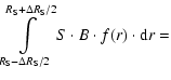$$\int\limits_{R_{\rm S}-\Delta R_{\rm S}/2}^{R_{\rm S}+\Delta R_{\rm S}/2}S\cdot B\cdot f(r)\cdot {\rm d}r= \frac{\pi}{180}\frac{\Psi \Delta R_{\rm S}B}{2-\alpha}\left[\left... ...{2-\alpha}-\left(R_{\rm S}-\frac{\Delta R_{\rm S}}{2} \right)^{2-\alpha}\right]$$

where S is area of the spot, and B is the spot's contrast (the spot-to-disk brightness ratio at the same distance from the white dwarf).

The results of testing have shown (Borisov & Neustroev 1998) that for a reliable estimation of the parameters it is important to keep the certain sequence of their determination. This is connected with the strong azimuth dependence of the emission line profile with variation of various spot parameters. When modelling the emission lines of IP Peg, we determined the parameters in the following order:

The orbital-phase modulation of the degree of asymmetry of the profile is used to find the phase angle of the spot $\vartheta$;

spectroscopic data are then sorted according to the "maximally effective'' phases for various parameters of the spot: the azimuthal extent of the spot $\Psi$ can be best determined at azimuths $-30^{\circ}$- $30^{\circ}$ and $150^{\circ}$- $210^{\circ}$, and the radial position of the spot R_S can be best determined at azimuths $50^{\circ }$- $130^{\circ}$ and $-50^{\circ }$- $-130^{\circ }$;

the azimuthal extent of the spot is determined, fixed, and then used in the estimation of the radial position of the spot in the accretion disk;

the remaining profiles are modelled with values of the already determined geometrical spot parameters fixed, in order to derive the relative luminosity of the spot at various orbital phases.

Figure 8: Accretion disk geometry for the line profile model described in the text.

 

 

Table 1: Average parameters of the accretion disk and the bright spot obtained by modelling separate spectra.

Emission	Dataset	$\alpha$	R	V	$\vartheta$	$\Psi$	$\Delta R_{\rm s}^{\ast}$	$R_{\rm s}$	Contrast
line
H$\beta$	First	1.67 $\pm$ 0.49	0.08 $\pm$ 0.04	570 $\pm$ 100	30	50 $\pm$ 15	0.1	0.95 $\pm$ 0.05	2.1 $\pm$ 1.5
H$\beta$	Second	1.61 $\pm$ 0.40	0.08 $\pm$ 0.03	590 $\pm$ 106	29	49 $\pm$ 18	0.1	0.96 $\pm$ 0.05	2.0 $\pm$ 1.1
H$\gamma$	First	2.15 $\pm$ 0.56	0.08 $\pm$ 0.03	549 $\pm$ 130	30	75 $\pm$ 6	0.1	0.90 $\pm$ 0.10	3.1 $\pm$ 2.6
H$\gamma$	Second	1.69 $\pm$ 0.47	0.08 $\pm$ 0.04	616 $\pm$ 102	26	42 $\pm$ 5	0.1	0.89 $\pm$ 0.08	4.9 $\pm$ 4.9
H$\delta$	First	1.68 $\pm$ 0.78	0.12 $\pm$ 0.06	669 $\pm$ 155	30	52 $\pm$ 16	0.1	0.88 $\pm$ 0.08	3.6 $\pm$ 3.2

$\parbox{15cm}{ $\ast$\space Adopted by default.}$

Since the shape of the profile is virtually independent of variations in the radial extent of the spot $\Delta R_{\rm S}$ (Borisov & Neustroev 1998), a default value for this parameter can be used in the profile computations (e.g., a typical radial extent of the bright spot). Photometric observations of the cataclysmic variables indicate that the radial extent of the spots vary from 0.02 to 0.15 (Rozyczka 1988). We adopted the value $\Delta R_{\rm S} = 0.1$.

The necessary condition for the accurate determination of the spot parameters is the knowledge of its phase angle $\vartheta$, which possibly can be found from the analysis of the phase variations of the degree of asymmetry of the emission line (S-wave graph). We must determine  $\varphi_{0}$. This phase corresponds to the moment when the radial velocity of the S-wave component is zero. Then the phase angle $\vartheta$of the spot will be $2 \pi (1 - \varphi _{0})$. Examples of the application of this technique to real data are given in Neustroev (1998) and Borisov & Neustroev (1999).

For the study of the accretion disk structure of IP Peg it was possible to apply this technique to all major emission lines (H$\alpha$, H$\beta$, H$\gamma$ and H$\delta$), but because of signal-to-noise limitations the discussion, following below, is mostly based on the H$\beta$ line. We have started our analysis of the spectroscopic data by determination of the phase angle $\vartheta$ of the spot, using the S-wave graph (Fig. 3). The value of $\vartheta$ has been found to be 30$^{\circ }$ (H$\beta$, H$\gamma$ and H$\delta$ lines from first dataset), 29$^{\circ }$ (the H$\beta$ line from second dataset) and 26$^{\circ }$ (the H$\gamma$ line from second dataset) respectively.

As a result of subsequent modelling we have established all principal parameters of the accretion disk and the bright spot. Their average values are listed in Table 1. It is necessary to note that the standard deviations of all averaged parameters of the disk are considerably higher than expected on the basis of testing (Borisov & Neustroev 1998). It may be due to possible orbital variations of the observed parameters of the accretion disk.

Figure 9: The dependence of the spot brightness on orbital phase, obtained from modelling of the H$\beta$ emission line. Obviously the brightness considerably oscillates, and during a significant part of the period the spot is not visible.