Up: Local velocity field from galaxies
Subsections
The method of sosie galaxies (Eq. (5)) does not correct for statistical
bias due to magnitude incompleteness (Malmquist bias). Two methods exist to detect
unbiased galaxies: the method of normalized distances (Bottinelli et al. 1986)
and the Spaenhauer diagram (Spaenhauer 1978) used by Sandage (1994).
A detailed discussion about
these methods is given by Teerikorpi (1997).
In the case of galaxies which are sosie
of a same calibrator, both diagrams are equivalent.
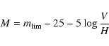
In order to correct for the Malmquist bias we have first to determine the actual
completeness limit of the apparent magnitudes.
The knowledge of the limiting apparent magnitude informs us about
galaxies missing at a given distance for a given absolute magnitude.
The construction of the curve  vs. apparent magnitude
(N is the number of galaxies brighter than the considered
apparent magnitude) is a classical way to estimate this limit.
If the distribution of galaxies is homogeneous, the slope expected is 0.6.
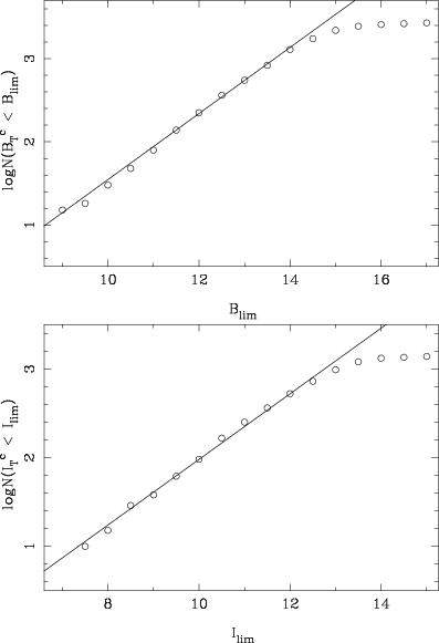
In Fig. 5 we show the completeness curves
for our sample, in B- and I-band respectively.
The limiting apparent magnitude is given where the curve begins to bend down.
vs. apparent magnitude
(N is the number of galaxies brighter than the considered
apparent magnitude) is a classical way to estimate this limit.
If the distribution of galaxies is homogeneous, the slope expected is 0.6.
In Fig. 5 we show the completeness curves
for our sample, in B- and I-band respectively.
The limiting apparent magnitude is given where the curve begins to bend down.
 |
Figure 5:
Completeness curve for the B and I-band apparent magnitudes. The
curve begins to bend down at  14 mag and 12.5 mag, respectively. 14 mag and 12.5 mag, respectively. |
The limiting apparent magnitude is
 mag in B and
 mag in I.
The slopes are
mag in I.
The slopes are
 and
and
 ,
for B and I respectively.
The result that the slope is smaller than the theoretical one has already been
discussed (Paturel et al. 1994; Teerikorpi et al. 1998).
In the following sections we will use the observed slope (0.4) and the limits
14 and 12.5 for B and I magnitudes.
,
for B and I respectively.
The result that the slope is smaller than the theoretical one has already been
discussed (Paturel et al. 1994; Teerikorpi et al. 1998).
In the following sections we will use the observed slope (0.4) and the limits
14 and 12.5 for B and I magnitudes.
The Spaenhauer diagram for galaxies which are sosie of a given calibrator is a
diagram of absolute magnitude against distance. From a practical
point of view, we are drawing the absolute magnitude versus the
radial velocity which is an estimate of the distance through the Hubble law,
after correction for the infall of our Local Group (hereafter LG) towards Virgo.
For this correction a preliminary infall velocity has been adopted
(200 km s-1). Eventually, it will be revised in forthcoming sections.
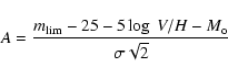
The construction of the Spaenhauer diagram requires three curves:
- 1.
- The curve showing the cut due to the limiting apparent magnitude.
We recall the equation of this curve:
 |
(6) |
where H is the adopted Hubble constant and
 the limiting apparent
magnitude, as defined in the previous section.
the limiting apparent
magnitude, as defined in the previous section.
- 2.
- The bias curve for a galaxy with a Gaussian absolute magnitude distribution
 is given by the equation (Teerikorpi 1975):
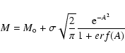 |
(7) |
with
 |
(8) |
and
 |
(9) |
- 3.
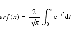
- The envelope of the distribution is given by the following equations
demonstrated in the Appendix A:
 |
(10) |
where  is the slope of the completeness curve divided by 0.2 (e.g.,
for the theoretical slope of 0.6 we expect
is the slope of the completeness curve divided by 0.2 (e.g.,
for the theoretical slope of 0.6 we expect  ). We assume that
  does not depend on the distance, but its value will be calculated at each step
of the iterative process. k depends on the adopted Hubble constant
and on the mean density of the considered galaxies.
Its expression is:
does not depend on the distance, but its value will be calculated at each step
of the iterative process. k depends on the adopted Hubble constant
and on the mean density of the considered galaxies.
Its expression is:
 |
(11) |
where V0.05 is the velocity at which the biased absolute magnitude is
changed by 5 percent. This level is arbitrarily chosen as the beginning of
the observable bias.
We construct the Spaenhauer diagram for each calibrator using our sample of
sosie galaxies. Let us recall that the adopted parameters are the following:
in B-band and 12.5 in I-band (Sect. 4.1).
From Fig. 5, we use the observed values
 for both B and I magnitudes.
We adopt provisionally a Local Group infall velocity of 200 km s-1
In a first step we start with a preliminary value of H and .
We adopted a starting dispersion
for both B and I magnitudes.
We adopt provisionally a Local Group infall velocity of 200 km s-1
In a first step we start with a preliminary value of H and .
We adopted a starting dispersion
 in B and
 in I and
a Hubble constant of 70 km s-1 Mpc-1
These values have no incidence on the final result.
They only affect the number of iterations.
We calculate the new H and
values from the unbiased galaxies
of the "plateau'' (i.e. galaxies with a velocity
less than V0.05)
in I and
a Hubble constant of 70 km s-1 Mpc-1
These values have no incidence on the final result.
They only affect the number of iterations.
We calculate the new H and
values from the unbiased galaxies
of the "plateau'' (i.e. galaxies with a velocity
less than V0.05)![[*]](/icons/foot_motif.gif) The new estimates are re-injected in a new iteration, and so on.
The calculation is stopped when H becomes stable.
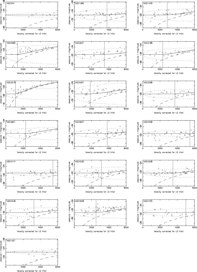
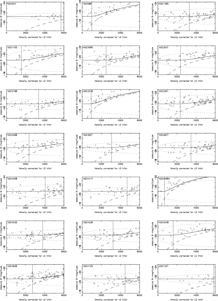
Figures 6 and 7 give the Spaenhauer diagrams in B and Ifor the 21 calibrators (two calibrators have no I-band magnitude).
It is interesting
to compare NGC 224 = M 31 and NGC 598 = M 33, the first two
galaxies in Fig. 6, because they represent two opposite cases:
one luminous galaxy (M 31) and one low luminosity one (M 33). The effect of the bias
is clearly visible.
The new estimates are re-injected in a new iteration, and so on.
The calculation is stopped when H becomes stable.
Figures 6 and 7 give the Spaenhauer diagrams in B and Ifor the 21 calibrators (two calibrators have no I-band magnitude).
It is interesting
to compare NGC 224 = M 31 and NGC 598 = M 33, the first two
galaxies in Fig. 6, because they represent two opposite cases:
one luminous galaxy (M 31) and one low luminosity one (M 33). The effect of the bias
is clearly visible.
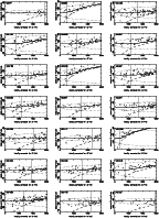 |
Figure 6:
Spaenhauer diagrams in B magnitudes. For each calibrator
we plot its sosie galaxies, with the predicted envelope (doted curve). The bias curve
is show as a solid curve. The region of completeness is above the dashed curve. Finally,
the unbiased region ("plateau'') is defined on the left of the vertical line.
The name of the calibrating galaxy is indicated in the upperleft corner of each frame. |
 |
Figure 7:
Spaenhauer diagrams in I magnitudes (same as Fig. 6). |
From the Spaenhauer diagram we extract the galaxies with a velocity below
V0.05. This is done for B and I separately. A mean distance
modulus is derived in B and I for each galaxy using Eq. (5):
The weighted mean distance modulus is then:
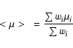 |
(12) |
where the weight (
 )
of each individual distance
modulus (
)
of each individual distance
modulus ( )
is calculated
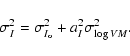
from the mean error on B or I magnitudes using the relations:
)
is calculated
from the mean error on B or I magnitudes using the relations:
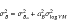 |
(13) |
 |
(14) |
Here aB=5.9 and aI=7.7 are the adopted slopes of the Tully-Fisher
relations in B and I, respectively. The mean errors
 ,
,
 and
and
 are taken from LEDA.
The mean error on the mean distance modulus is then:
 |
(15) |
The list of 283 unbiased galaxies is given in Table 2
with the following parameters:
Column 1: PGC number from LEDA.
Column 2: Alternate name from LEDA.
Column 3: Right Ascension and declination for equinox 2000 in hours,
minutes, seconds and tenth and degrees, arcminute and arcseconds.
Column 4: Radial velocity corrected for a preliminary infall velocity
of the LG towards Virgo (
 km s-1).
Column 5: Weighted mean distance modulus and its mean error. The merging
of B and I bands is given in Fig. 8.
Column 6: Angular distance from the Virgo center. The center of Virgo
is placed on M 87 at equatorial coordinates of
J123049.2+122329.
We can now start the study of the local velocity field around Virgo from
this unbiased sample.
Up: Local velocity field from galaxies
Copyright ESO 2002