Distribution functions of intensities and velocities in the data cubes are shown in Fig. 2. Intensity and velocity histograms of all pixels in the time series are plotted. At first glance the velocities seem to be symmetrically distributed around zero - this is partially caused by the definition of the zero points in the velocity maps (see Sect. 2) - but the curves do not have exact Gaussian shapes as found e.g. by Keil & Canfield (1978). The slopes towards negative velocities are significantly steeper than towards positive velocities. The maxima of the curves are at -125 m s-1 (for v0) and at -145 m s-1 (for v50), respectively. As already shown in Hirzberger et al. (2001) the velocity fluctuations exhibit only a small variation with photospheric height. The FWHM of the two curves are 1.125 km s-1 (for v0) and 1.380 km s-1 (for v50). A further conclusion extracted from the velocity distributions is that the upflow and downflow areas are almost equal. The fractional area of positive velocities (upflows) amounts to 48.6% (for v0) and to 49.0% (for v50). Both values are rather close to the fractional granular area detected by the applied image segmentation algorithm (see Sect. 3 above).
The distribution functions of the intensities (lower panel of
Fig. 2) show considerable variations with photospheric height.
The curve corresponding to I0 is almost symmetrical with a
maximum at 0.998 and a FWHM of 0.098. In deeper photospheric
levels the curves become broader - i.e. the rms contrasts are
increasing - and the maxima of the curves are shifted to lower
values. For I50 the maximum of the distribution function is
located at 0.978 (
FWHM=0.149) and that for
![]() is at 0.948
(
FWHM=0.232). The detected asymmetries of the distribution
functions can also be seen in results from numerical simulations
(Stein & Nordlund 1998) and do not imply that the ratios of areas
brighter and fainter than the average values have to deviate
significantly from one. The fractions of areas brighter than the
mean intensities are 49.4% (for I0), 47.1% (for I50),
and 47.0% (for
is at 0.948
(
FWHM=0.232). The detected asymmetries of the distribution
functions can also be seen in results from numerical simulations
(Stein & Nordlund 1998) and do not imply that the ratios of areas
brighter and fainter than the average values have to deviate
significantly from one. The fractions of areas brighter than the
mean intensities are 49.4% (for I0), 47.1% (for I50),
and 47.0% (for
![]() ).
).
An adequate method for describing shapes of structures is the calculation of structural parameters. The distributions of four such structural parameters are plotted in Fig. 3. They have been defined, according to Stoyan & Stoyan (1992), as follows:
The area-perimeter factor,
![]() ,
denotes the ratio
of a perimeter calculated from the area, A, of the structure
assuming a circular shape and the actual perimeter, P.
,
denotes the ratio
of a perimeter calculated from the area, A, of the structure
assuming a circular shape and the actual perimeter, P.
 |
(1) |
The circularity factor, ![]() ,
denotes the ratio of a diameter
calculated from the area of the structure assuming circularity and the
so-called maximum Feret-diameter,
,
denotes the ratio of a diameter
calculated from the area of the structure assuming circularity and the
so-called maximum Feret-diameter, ![]() ,
which corresponds to the
maximum distance of two points on the boundary of the analyzed
structure.
,
which corresponds to the
maximum distance of two points on the boundary of the analyzed
structure.
 |
(2) |
| (3) |
| (4) |
![\begin{displaymath}a=\xi +\left[\xi^2-\frac{A}{\pi}\right]^{1/2}\quad\mbox{with}...
...{3}\left[\left(\frac{A}{\pi}\right)^{1/2}+\frac{P}{\pi}\right]
\end{displaymath}](/articles/aa/full/2002/36/aah3646/img63.gif)
Figure 3 shows the distribution of the four previously defined
structural parameters calculated for granules and granular cells. The
distributions corresponding to the granules are generally broader
than those for the granular cells. Especially the distributions of
![]() exhibit completely different shapes. The curve for the
granular cells shows almost a Gaussian distribution around 0.5
reflecting that the cells have mainly regular shapes. Their
perimeters are by a factor
exhibit completely different shapes. The curve for the
granular cells shows almost a Gaussian distribution around 0.5
reflecting that the cells have mainly regular shapes. Their
perimeters are by a factor ![]() longer than expected for a
circle. The distribution for the granules has its maximum at
longer than expected for a
circle. The distribution for the granules has its maximum at
![]() and a long tail up to values of
and a long tail up to values of
![]() .
Hence,
most of the granules have extremely complex shapes but, however, a
quite large number of them - mainly very small granules whose
perimeters might be artificially shortened by the finite pixel size
of the data - are rather regularly shaped.
.
Hence,
most of the granules have extremely complex shapes but, however, a
quite large number of them - mainly very small granules whose
perimeters might be artificially shortened by the finite pixel size
of the data - are rather regularly shaped.
For ![]() the differences between granules and granular cells are
not so large, yet still significant. Both distributions have a
well-defined maximum and broad tails on both sides of it. The big
difference between the distributions of
the differences between granules and granular cells are
not so large, yet still significant. Both distributions have a
well-defined maximum and broad tails on both sides of it. The big
difference between the distributions of ![]() and
and
![]() for
granules means that it is true that the granules have mainly very
complex boundaries but their overall shapes do not deviate much
from being circular.
for
granules means that it is true that the granules have mainly very
complex boundaries but their overall shapes do not deviate much
from being circular.
The last statement has to be weakened when looking at the
distribution functions of ![]() .
Both curves cover almost the entire
range between 0 and 1. Clearly defined maxima are not visible although
the curves converge rather fast to zero below
.
Both curves cover almost the entire
range between 0 and 1. Clearly defined maxima are not visible although
the curves converge rather fast to zero below
![]() (granules)
and
(granules)
and
![]() (granular cells). Hence, most granules might have
overall regular shapes (large
(granular cells). Hence, most granules might have
overall regular shapes (large ![]() )
with irregular boundaries
(leading to a low
)
with irregular boundaries
(leading to a low
![]() )
but their overall shapes are significantly
elongated and not circular. The peak at
)
but their overall shapes are significantly
elongated and not circular. The peak at
![]() for granules is an
artefact due to the finite pixel size yielding many structures whose
lengths are exactly twice as long as their widths.
for granules is an
artefact due to the finite pixel size yielding many structures whose
lengths are exactly twice as long as their widths.
The ellipticity factor ![]() is extremely low for all structures,
granules and granular cells. Hence, the granules do have rather
elongated shapes but the shapes are far from being elliptical.
is extremely low for all structures,
granules and granular cells. Hence, the granules do have rather
elongated shapes but the shapes are far from being elliptical.
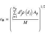
The broad band intensities and velocities (from level ![]() )
were averaged within each of the 5509 granules detected in the
time series. Their dependence on the granular size is plotted in
Fig. 4, in which the effective granular diameter,
)
were averaged within each of the 5509 granules detected in the
time series. Their dependence on the granular size is plotted in
Fig. 4, in which the effective granular diameter, ![]() ,
is defined
assuming circular shapes:
,
is defined
assuming circular shapes:
![]() .
.
The average granular intensities,
![]() ,
show an
increase for small radii and remain nearly constant for granules
larger than approximately
,
show an
increase for small radii and remain nearly constant for granules
larger than approximately
![]() .
Qualitatively this is in
good agreement with former results found in Hirzberger et al.
(1997) and Berrilli et al. (2002) and does also agree with numerical
simulations of Gadun et al. (2000). However, the position of the
elbow is slightly shifted to smaller granules as found in the above
cited references. This might be a consequence of the excellent
spatial resolution of the data since the image segmentation
algorithm used here is the same as applied in Hirzberger et al.
(1997). In the lower panel of Fig. 4 the corresponding mean granular
velocities,
.
Qualitatively this is in
good agreement with former results found in Hirzberger et al.
(1997) and Berrilli et al. (2002) and does also agree with numerical
simulations of Gadun et al. (2000). However, the position of the
elbow is slightly shifted to smaller granules as found in the above
cited references. This might be a consequence of the excellent
spatial resolution of the data since the image segmentation
algorithm used here is the same as applied in Hirzberger et al.
(1997). In the lower panel of Fig. 4 the corresponding mean granular
velocities,
![]() ,
are shown. Their dependence on
the granular radius agrees almost perfectly with that of the broad
band intensities.
,
are shown. Their dependence on
the granular radius agrees almost perfectly with that of the broad
band intensities.
A conspicuous result to be noticed in Fig. 4 is that the distributions
of both parameters, average granular intensities and velocities, do
not increase monotonically with ![]() ,
i.e. the maximum values can be
found in the range
,
i.e. the maximum values can be
found in the range
![]() .
This is in contrast
to the distribution of the maximum granular intensities and velocities
(not shown) which converge monotonically to asymptotic values (see
also Figs. 12 and 13 in Berrilli et al. 2002). Therefore, granules
larger than about
.
This is in contrast
to the distribution of the maximum granular intensities and velocities
(not shown) which converge monotonically to asymptotic values (see
also Figs. 12 and 13 in Berrilli et al. 2002). Therefore, granules
larger than about
![]() must have a rich internal structure
containing very bright regions but also rather dark regions leading to
a reduction of the average granular intensity. This conclusion is
quite obvious when looking at a granular image, e.g. the one shown in
Fig. 1. Also the development of dark centers in large granules is well
known for many years. According to numerical simulations (e.g. Stein & Nordlund 1998; Gadun et al. 2000) this arises from a pressure
excess developing above large granules which reduces the upflow velocity
and, consequently, the transport of thermal energy from below.
The evident close similarity of the two distributions shown in Fig. 4
is, thus, well supported by theoretical models.
must have a rich internal structure
containing very bright regions but also rather dark regions leading to
a reduction of the average granular intensity. This conclusion is
quite obvious when looking at a granular image, e.g. the one shown in
Fig. 1. Also the development of dark centers in large granules is well
known for many years. According to numerical simulations (e.g. Stein & Nordlund 1998; Gadun et al. 2000) this arises from a pressure
excess developing above large granules which reduces the upflow velocity
and, consequently, the transport of thermal energy from below.
The evident close similarity of the two distributions shown in Fig. 4
is, thus, well supported by theoretical models.
The average granular intensities and velocities from higher
photospheric levels,
![]() and
and
![]() ,
are plotted in Fig. 5 vs. those from
lower photospheric heights. The correlation between
,
are plotted in Fig. 5 vs. those from
lower photospheric heights. The correlation between
![]() and
and
![]() is nearly perfect
and independent on the granular radius. The slope of the distribution
is only slightly smaller than unity which means that the average
velocities do not decrease significantly in the probed height
interval. The same is valid for the maximum velocities which are not
shown here.
is nearly perfect
and independent on the granular radius. The slope of the distribution
is only slightly smaller than unity which means that the average
velocities do not decrease significantly in the probed height
interval. The same is valid for the maximum velocities which are not
shown here.
The correlation between
![]() and
and
![]() is not that good as found for the velocities and
the correlation is considerably lower for small granules than for
larger ones. This is due to several reasons: (i) The overall scatter
is significantly larger as for the velocities; (ii) the slope of the
distributions is significantly steeper for larger granules than for
smaller ones. Thus, smaller granules exhibit in average a much faster
reduction of their intensity with photospheric height than larger
ones; (iii) some small structures exhibit an extremely high line
center intensity. Possibly, these are magnetic structures which
additionally bias the correlation between
is not that good as found for the velocities and
the correlation is considerably lower for small granules than for
larger ones. This is due to several reasons: (i) The overall scatter
is significantly larger as for the velocities; (ii) the slope of the
distributions is significantly steeper for larger granules than for
smaller ones. Thus, smaller granules exhibit in average a much faster
reduction of their intensity with photospheric height than larger
ones; (iii) some small structures exhibit an extremely high line
center intensity. Possibly, these are magnetic structures which
additionally bias the correlation between
![]() and
and
![]() .
.
It can be concluded from Fig. 5 that large granules exhibit an intensity excess also at higher photospheric levels whereas smaller granules dissolve at much lower heights. Hence, this result agrees partially with those found in Komm et al. (1991) that the typical length scale of intensity variations increases with photospheric height. For granular velocities this variation cannot be detected which contradicts the result of Komm et al. (1991).
In Sect. 4.3 it was pointed out that (at least large) granules
must have a rich internal intensity and velocity structure. Thus,
an interesting question is how the intensities and
velocities are distributed within the granules. As a first
approximation to answer this question, the distances between
the granular barycenters,
![]() ,
defined as
,
defined as
 |
(5) |
It is evident from the distributions plotted in Fig. 6 that for small granules the maximum intensities as well as the maximum velocities are located much closer to the granule barycenters as for larger ones. The dependences on the granular radius show nearly linear trends. This result confirms statistically the results of e.g. Nesis et al. (1992) or Krieg et al. (2000) who claimed that the maximum granular intensities and velocities tend to be located close to the granule boundaries although this claim seems to be valid only for very large granules. This result also agrees well with numerical models of Rast (1995) in which the fastest and brightest granular regions are locations of displaced material when fast downdrafts develop. Therefore, the fastest and brightest granular regions are located close to the intergranular lanes, i.e. at the granular boundaries.
The very large relative distances,
![]() and
and
![]() which can be found in Fig. 6 do not
mean that the brightest pixels are located outside the granule,
i.e. that the segmentation algorithm is not working properly. This
is rather due to the very complex granular shapes, e.g.
corresponding to elongation factors far below
which can be found in Fig. 6 do not
mean that the brightest pixels are located outside the granule,
i.e. that the segmentation algorithm is not working properly. This
is rather due to the very complex granular shapes, e.g.
corresponding to elongation factors far below
![]() (see Fig. 3).
(see Fig. 3).
The location of pixels with maximum intensities and velocities has
low statistical significance in cases where granules have areas of
several hundred pixels. Moreover, the distribution shown in the middle
panel of Fig. 6 seems to be also biased by a residual distortion
between broad band images and velocity maps. This can be seen in the
region
![]() and
and
![]() where many displacements are
found. For these tiny granules the detected shapes from the broad band
images might be somewhat distorted with respect to the velocity maps.
This is a consequence of the limited spatial resolution of the narrow
band data which is in the range of
where many displacements are
found. For these tiny granules the detected shapes from the broad band
images might be somewhat distorted with respect to the velocity maps.
This is a consequence of the limited spatial resolution of the narrow
band data which is in the range of
![]() ,
and thus approximately
4 pixels (see Hirzberger et al. 2001).
,
and thus approximately
4 pixels (see Hirzberger et al. 2001).
To overcome this problem and to increase the statistical
significance of the measured intensity and velocity structure
within the granules, "inertial radii'',
![]() ,
can
be defined from the moment of inertia around a vertical axis
through the granular barycenters. For convenience, i.e. to
include also the structure of the intergranular lanes
surrounding the granules,
,
can
be defined from the moment of inertia around a vertical axis
through the granular barycenters. For convenience, i.e. to
include also the structure of the intergranular lanes
surrounding the granules,
![]() has been computed from
the entire granular cells including granular and intergranular
regions as defined in Sect. 3.
has been computed from
the entire granular cells including granular and intergranular
regions as defined in Sect. 3.
 |
(6) |
Figure 7 (upper panel) shows area inertial radii, ![]() ,
i.e.
assuming that the density
,
i.e.
assuming that the density ![]() is constant in the granular
cell, for the 5509 detected granules vs. the granule
radius. The absolute
is constant in the granular
cell, for the 5509 detected granules vs. the granule
radius. The absolute ![]() have been normalized to the cell radii,
have been normalized to the cell radii,
![]() .
The distribution shows no clear trend.
For most of the small granules the relative area inertial radius,
.
The distribution shows no clear trend.
For most of the small granules the relative area inertial radius,
![]() ,
lies in the range between 0.8 and 1. For the sake of
comparison, the inertial radius (assuming constant density) for a
circle with radius R is
,
lies in the range between 0.8 and 1. For the sake of
comparison, the inertial radius (assuming constant density) for a
circle with radius R is
![]() and for a rectangle
with a side ratio of 1/3 the relative area inertial radius is
and for a rectangle
with a side ratio of 1/3 the relative area inertial radius is
![]() .
For larger structures the
.
For larger structures the
![]() scatter is in a range between 0.75 and 1.4
although a slight tendency for a general decrease of
scatter is in a range between 0.75 and 1.4
although a slight tendency for a general decrease of
![]() with
with ![]() can be detected. This means
that most of the large granular cells are more roundish than smaller
ones - this might be slightly biased by the finite pixel size - but
some of them (those with
can be detected. This means
that most of the large granular cells are more roundish than smaller
ones - this might be slightly biased by the finite pixel size - but
some of them (those with
![]() )
must have very
elongated shapes, too.
)
must have very
elongated shapes, too.
The lower panel of Fig. 7 shows ratios between the broad band
inertial radii of the granular cells,
![]() ,
and the area inertial
radii. The
,
and the area inertial
radii. The
![]() have been calculated setting
have been calculated setting
![]() in
Eq. (6). For very small granules with
in
Eq. (6). For very small granules with
![]() the ratio
increases with decreasing size, achieving values larger than
0.9 for the tiniest structures. Hence, these granules must have an
almost homogeneous intensity structure (
the ratio
increases with decreasing size, achieving values larger than
0.9 for the tiniest structures. Hence, these granules must have an
almost homogeneous intensity structure (
![]() for constant
for constant
![]() ). Of course the ratio does not achieve unity because the
intergranular lanes around these small granules reduces
). Of course the ratio does not achieve unity because the
intergranular lanes around these small granules reduces
![]() compared to
compared to ![]() .
For granules in the range
.
For granules in the range
![]() the
ratio of inertial radii exhibits a clear minimum. For these granules
bright intensity maxima must exist close to their barycenters.
For granules larger than
the
ratio of inertial radii exhibits a clear minimum. For these granules
bright intensity maxima must exist close to their barycenters.
For granules larger than
![]() the ratio
increases with the granule radius, i.e. the larger the granules are
the closer the brightest regions are situated to the granule
boundaries. This result is in good agreement with Fig. 6 but has a
much higher statistical significance.
the ratio
increases with the granule radius, i.e. the larger the granules are
the closer the brightest regions are situated to the granule
boundaries. This result is in good agreement with Fig. 6 but has a
much higher statistical significance.
In Fig. 8 intensity inertial radii computed from the broad band
images and the intensity maps together with velocity inertial radii
computed from the velocity maps are plotted vs. ![]() .
The
absolute inertial radii,
.
The
absolute inertial radii,
![]() ,
,
![]() ,
,
![]() ,
,
![]() ,
and
,
and
![]() have been normalized to the area
inertial radius
have been normalized to the area
inertial radius ![]() of each cell. For the sake of an easier representation the resulting
ratios have been averaged in overlapping bins of
of each cell. For the sake of an easier representation the resulting
ratios have been averaged in overlapping bins of
![]() width
(moving window method). This method using overlapping bins
has the advantage that the averaged curves additionally become
effectively smoothed. Qualitatively, all the curves plotted in Fig. 8
have the same shapes, i.e. they are close to one for the very smallest
and very largest granules and have a minimum at intermediate
granular radii. The two curves calculated from the velocity maps
(v0 and v50) are almost identical, i.e. the velocity
structure does not change in the probed photospheric height interval.
The curve derived from I0 deviates significantly from the others:
(i) the minimum is shifted to larger granules (
width
(moving window method). This method using overlapping bins
has the advantage that the averaged curves additionally become
effectively smoothed. Qualitatively, all the curves plotted in Fig. 8
have the same shapes, i.e. they are close to one for the very smallest
and very largest granules and have a minimum at intermediate
granular radii. The two curves calculated from the velocity maps
(v0 and v50) are almost identical, i.e. the velocity
structure does not change in the probed photospheric height interval.
The curve derived from I0 deviates significantly from the others:
(i) the minimum is shifted to larger granules (
![]() )
and (ii) the minimum is much shallower than those of the other three
curves. The shift of the minimum can be explained by the fact that the
intensity excess of smaller granules dissolves at lower photospheric
heights than that of larger ones (see also Fig. 5). The shallow
minimum is due to the much lower rms intensity fluctuations measured
in I0 compared to those in I50 and
)
and (ii) the minimum is much shallower than those of the other three
curves. The shift of the minimum can be explained by the fact that the
intensity excess of smaller granules dissolves at lower photospheric
heights than that of larger ones (see also Fig. 5). The shallow
minimum is due to the much lower rms intensity fluctuations measured
in I0 compared to those in I50 and
![]() (see
Hirzberger et al. 2001).
(see
Hirzberger et al. 2001).
For the very smallest granules the ratio of the inertial radii
approaches almost one for the curves derived from I0,
I50, v0, and v50, respectively, whereas the curve
corresponding to
![]() reaches only 0.92. This might be
explained by a residual distortion of the intensity and velocity maps
compared to the broad band images. Hence, the granular cells detected
in the broad band images are not exactly co-aligned with the
corresponding granules in the intensity and velocity maps. However,
this effect becomes crucial only for the very smallest structures with
reaches only 0.92. This might be
explained by a residual distortion of the intensity and velocity maps
compared to the broad band images. Hence, the granular cells detected
in the broad band images are not exactly co-aligned with the
corresponding granules in the intensity and velocity maps. However,
this effect becomes crucial only for the very smallest structures with
![]() because for these structures the expected
residual distortion - which is in the range of the expected spatial
resolution of the narrow band data, i.e., approximately
because for these structures the expected
residual distortion - which is in the range of the expected spatial
resolution of the narrow band data, i.e., approximately
![]() -
is in the range of the sizes of the granules.
-
is in the range of the sizes of the granules.
![\begin{figure}
\par\includegraphics[width=8.8cm,clip]{h3646f9.eps} \end{figure}](/articles/aa/full/2002/36/aah3646/img116.gif) |
Figure 9:
Two-dimensional - azimuthally averaged along circles of
constant wavenumbers
|
The result from the previous section - highest intensities and
velocities are located close to the granular boundaries - implies
a sharp transition of both parameters from the granules to the
intergranular lanes, i.e. high horizontal intensity and
velocity gradients. In the lower panel of Fig. 1 an example of the
broad band intensity gradient,
![]() ,
is
displayed. The derivatives have been calculated using a three
point Lagrangian interpolation algorithm. The structures visible
in this image coincide, as expected, well with the contours of the
granules. At first glance it seems that all visible structures
have the same width of about
,
is
displayed. The derivatives have been calculated using a three
point Lagrangian interpolation algorithm. The structures visible
in this image coincide, as expected, well with the contours of the
granules. At first glance it seems that all visible structures
have the same width of about
![]() which means that the
width of the transition zone between granules and intergranular
lanes is independent on the size and the intensity of the granules.
which means that the
width of the transition zone between granules and intergranular
lanes is independent on the size and the intensity of the granules.
Figure 9 shows power spectra of the broad band image and of the
gradient map displayed in Fig. 1. For structures with diameters,
![]() ,
the power spectrum of the broad band image
falls nearly exponentially to zero (for a discussion of the power
laws of granulation images see e.g. Espagnet et al. 1993; Hirzberger
et al. 1997; Nordlund et al. 1997) whereas the power spectrum of
the gradient image shows a linear decrease down to a wavenumber of
approximately k=17 Mm-1 (
,
the power spectrum of the broad band image
falls nearly exponentially to zero (for a discussion of the power
laws of granulation images see e.g. Espagnet et al. 1993; Hirzberger
et al. 1997; Nordlund et al. 1997) whereas the power spectrum of
the gradient image shows a linear decrease down to a wavenumber of
approximately k=17 Mm-1 (
![]() ). Since the structures
visible in the gradient image (Fig. 1) are mainly thin and elongated,
this result can be interpreted such that it is dominated by structures
with a maximum length of approximately
). Since the structures
visible in the gradient image (Fig. 1) are mainly thin and elongated,
this result can be interpreted such that it is dominated by structures
with a maximum length of approximately
![]() (k=2.17 Mm-1) and with a minimum extension or typical width
of
(k=2.17 Mm-1) and with a minimum extension or typical width
of
![]() .
.
In the upper panel of Fig. 10 the maximum gradient of the broad band intensity in each of the 5509 granular cells (granules plus surrounding intergranular lanes) vs. the maximum broad band intensity in each granular cell is plotted. In the lower panel of Fig. 10 the maximum gradients of the velocities (i=50%) vs. the maximum velocities in the granules are shown. Both plots exhibit a clear and nearly linear trend although the lower one is tainted with somewhat higher scatter resulting in a flattening of the trend for structures with maximum velocities below zero. These latter structures do have maximum intensities below one, i.e. they are small structures which seem to be slightly affected by some residual noise in the velocity maps.
The appearance of the linear trends in Fig. 10 means that brighter granules and granules containing faster upflows show a steeper drop of intensity and velocity towards the intergranular lanes than fainter ones. This follows from the fact that (i) the brighter the granules are the closer the location of the maximum intensities and velocities is situated to the granular boundary and (ii) that the width of the structures found in the gradient images (e.g. the one in Fig. 1) is independent on the granular size or intensity. However, this result does not mean that the brightest granules must be surrounded by the darkest intergranular lanes. Plotting maximum granular broad band intensities vs. minimum intergranular broad band intensities (not shown) exhibits a slight negative trend but with a correlation of only -0.21. The correlation between maximum granular velocities and minimum intergranular velocities is, with -0.18 (for i=0%) and with -0.16 (for i=50%), even weaker.
In the present data the time interval between two images is
70 s, which is in the range of the lifetimes of small granules
(see Hirzberger et al. 1999). Hence, for studying the temporal
evolution of the granulation pattern a direct tracking of
individual structures is not possible. An alternative attempt is
shown in Fig. 11. In this figure, the temporal variation of
the coherence spectra of broad band images and line center
intensity maps are plotted. The coherence spectrum, C(k), of
two images, F(x,y) and G(x,y), is defined as
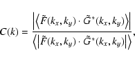 |
(7) |
![\begin{figure}
\par\includegraphics[width=18cm,clip]{fig11.eps} \end{figure}](/articles/aa/full/2002/36/aah3646/img124.gif) |
Figure 11:
Averaged coherence spectra of broad band images
(left panel) and of line core intensity maps
(right panel). The parameter |
The columns in the images shown in Fig. 11 denote averages
of coherence spectra, C(tm,k), from images, Fl and Fl+m,
separated by a constant time interval
![]() :
:
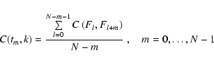 |
(8) |
Figure 11, hence, shows the temporal variation of the coherence of
the granulation pattern in dependence on the structural sizes.
In the left panel (broad band data) the coherence is
high in the region around k=5 Mm-1 (
![]() )
and for
)
and for
![]() min which denotes typical sizes and lifetimes of
large granules. For smaller structures
(5 Mm
-1<k<20 Mm-1) the time interval of high
coherences drops quickly to zero. For smaller wavenumbers the same
is valid but the coherence shows additional peaks at
min which denotes typical sizes and lifetimes of
large granules. For smaller structures
(5 Mm
-1<k<20 Mm-1) the time interval of high
coherences drops quickly to zero. For smaller wavenumbers the same
is valid but the coherence shows additional peaks at
![]() min and at
min and at
![]() min for k=1.6 Mm-1
and at
min for k=1.6 Mm-1
and at
![]() min for k=0.7 Mm-1. A slight increase of
the coherence is also visible at k=3.8 Mm-1 and
30 min <tm<40 min. These secondary peaks might be resulting from
large and recurrent exploding granules first detected by Carlier et al. (1968) or from strong positive divergences (SPDs) found by
Rieutord et al. (2000). Meso- and supergranular structures are
expected to have longer lifetimes than the time intervals between
these secondary peaks. Moreover, they should not be visible that
clearly in the broad band data although it has to be assumed
that the positions where recurrent granules are situated are somehow
related to those large-scale flow fields (see e.g. Oda 1984; Title
et al. 1989). Yet, a detailed study of these structures visible in
the very low k-range is not the aim of the present work because of
the limited field of view yielding a rather low wavenumber resolution
in the range below k=3 Mm-1.
min for k=0.7 Mm-1. A slight increase of
the coherence is also visible at k=3.8 Mm-1 and
30 min <tm<40 min. These secondary peaks might be resulting from
large and recurrent exploding granules first detected by Carlier et al. (1968) or from strong positive divergences (SPDs) found by
Rieutord et al. (2000). Meso- and supergranular structures are
expected to have longer lifetimes than the time intervals between
these secondary peaks. Moreover, they should not be visible that
clearly in the broad band data although it has to be assumed
that the positions where recurrent granules are situated are somehow
related to those large-scale flow fields (see e.g. Oda 1984; Title
et al. 1989). Yet, a detailed study of these structures visible in
the very low k-range is not the aim of the present work because of
the limited field of view yielding a rather low wavenumber resolution
in the range below k=3 Mm-1.
The coherence spectra of the line core intensity maps (right panel of Fig. 11) show a gap in the region 4 min <tm<10 min and 1 Mm-1<k<3 Mm-1. It can be concluded from this result that granules are almost completely dissolved at this photospheric height (320 km). Smaller structures are clearly visible and seem to have quite long lifetimes of more than 10 min. These structures cannot be granules because small ones should dissolve at much lower photospheric heights than larger ones. Possibly, the origin of the high coherence in that region are magnetic structures which become bright in high photospheric levels. In the line core maps a few of these structures are visible but their number is very small (see also Fig. 5) so that they do not considerably bias the statistics carried out in the previous sections.
The secondary peaks at k=1.6 Mm-1 (
![]() min
and
min
and
![]() min) and k=0.7 Mm-1 (
min) and k=0.7 Mm-1 (
![]() min)
are also visible in the line core coherence spectra but the
increase of coherence at k=3.8 Mm-1 has almost disappeared.
Since broad band and narrow band data are obtained from independent
observations, the secondary peaks should represent real physical
phenomena. The very largest and brightest exploding granules which
might be responsible for these secondary peaks are expected to
produce positive temperature and brightness excesses also at high
photospheric levels (see e.g. Roudier et al. 2001). Thus, it is not
surprising that they are also visible in the line core data.
min)
are also visible in the line core coherence spectra but the
increase of coherence at k=3.8 Mm-1 has almost disappeared.
Since broad band and narrow band data are obtained from independent
observations, the secondary peaks should represent real physical
phenomena. The very largest and brightest exploding granules which
might be responsible for these secondary peaks are expected to
produce positive temperature and brightness excesses also at high
photospheric levels (see e.g. Roudier et al. 2001). Thus, it is not
surprising that they are also visible in the line core data.
It is possible to obtain lifetimes of granular features from the
coherence spectra shown in Fig. 11. In Fig. 12 e-folding times,
![]() ,
i.e. the times, tm, in which the coherences fall below
1/e, vs. k are plotted. To overcome the relatively low
temporal resolution of the analyzed data (70 s cadence between two
images) the coherences have been interpolated using cubic splines before
calculating the e-folding times. The curves are nearly identical
for all the used data, except the curve corresponding to the line
core intensity maps deviates slightly from the others. The e-folding
times of the remaining parameters show well defined maxima at
,
i.e. the times, tm, in which the coherences fall below
1/e, vs. k are plotted. To overcome the relatively low
temporal resolution of the analyzed data (70 s cadence between two
images) the coherences have been interpolated using cubic splines before
calculating the e-folding times. The curves are nearly identical
for all the used data, except the curve corresponding to the line
core intensity maps deviates slightly from the others. The e-folding
times of the remaining parameters show well defined maxima at
![]() Mm-1 and a quite noisy behaviour for smaller k.
This noisy character is probably caused by a combination of two
effects: (i) the poor resolution in the low k-range and (ii) due
to the large variety of phenomena in this range, e.g. large exploding
granules (recurrent and non-recurring), SPDs, meso- and supergranules,
etc.
Mm-1 and a quite noisy behaviour for smaller k.
This noisy character is probably caused by a combination of two
effects: (i) the poor resolution in the low k-range and (ii) due
to the large variety of phenomena in this range, e.g. large exploding
granules (recurrent and non-recurring), SPDs, meso- and supergranules,
etc.
In the range k>3.5 Mm-1 the e-folding times exhibit
an almost perfect linear (in this log-log representation) decrease
from
![]() min down to the time interval between two images
in the time series is reached, which takes place at
min down to the time interval between two images
in the time series is reached, which takes place at
![]() Mm-1. The linearity continues slightly below
Mm-1. The linearity continues slightly below
![]() s which is caused by the spline interpolation of the
measured coherences. The inset in Fig. 12 shows once more the
e-folding times for the broad band images (in the range
3.2 Mm
-1<k<20.5 Mm-1). The overplotted linear fit
represents a power law of the form
s which is caused by the spline interpolation of the
measured coherences. The inset in Fig. 12 shows once more the
e-folding times for the broad band images (in the range
3.2 Mm
-1<k<20.5 Mm-1). The overplotted linear fit
represents a power law of the form
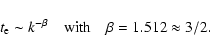 |
(9) |
Copyright ESO 2002
![\begin{figure}
\par\includegraphics[width=8.8cm,clip]{h3646f2.eps} \end{figure}](/articles/aa/full/2002/36/aah3646/img52.gif)
![\begin{figure}
\par\includegraphics[width=8.8cm,clip]{h3646f3.eps} \end{figure}](/articles/aa/full/2002/36/aah3646/img65.gif)
![\begin{figure}
\par\includegraphics[width=8.8cm,clip]{h3646f4.eps} \end{figure}](/articles/aa/full/2002/36/aah3646/img73.gif)
![\begin{figure}
\par\includegraphics[width=17.4cm,clip]{h3646f5.eps} \end{figure}](/articles/aa/full/2002/36/aah3646/img81.gif)
![\begin{figure}
\par\includegraphics[width=8.8cm,clip]{h3646f6.eps} \end{figure}](/articles/aa/full/2002/36/aah3646/img88.gif)
![\begin{figure}
\par\includegraphics[width=8.8cm,clip]{fig7.eps} \end{figure}](/articles/aa/full/2002/36/aah3646/img93.gif)
![\begin{figure}
\par\includegraphics[width=17.5cm,clip]{fig8.eps} \end{figure}](/articles/aa/full/2002/36/aah3646/img105.gif)
![\begin{figure}
\par\includegraphics[width=8.8cm,clip]{fig10.eps} \end{figure}](/articles/aa/full/2002/36/aah3646/img117.gif)
![\begin{figure}
\par\includegraphics[width=17.2cm,clip]{fig12.eps} \end{figure}](/articles/aa/full/2002/36/aah3646/img133.gif)