2 Observations, reductions and calibrations

2.1 Pre-reduction of the images

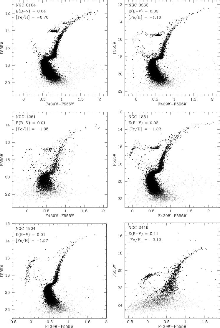
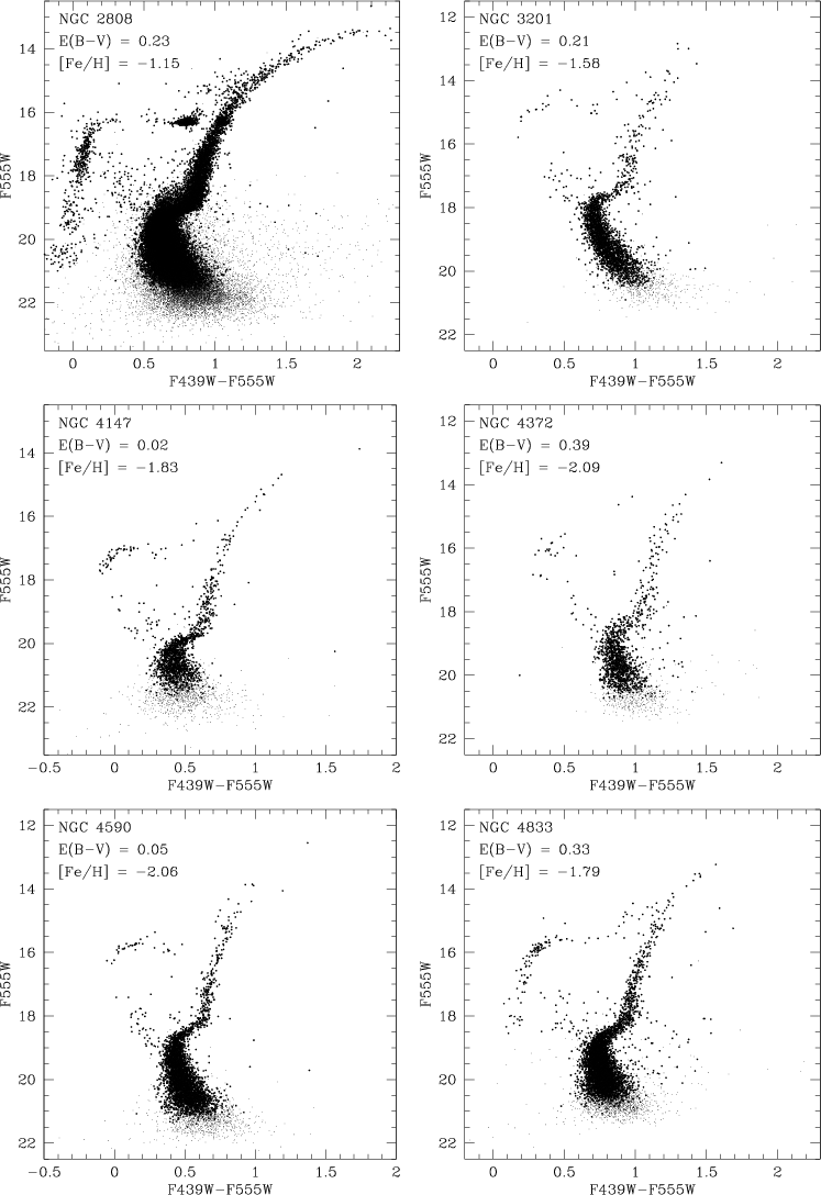
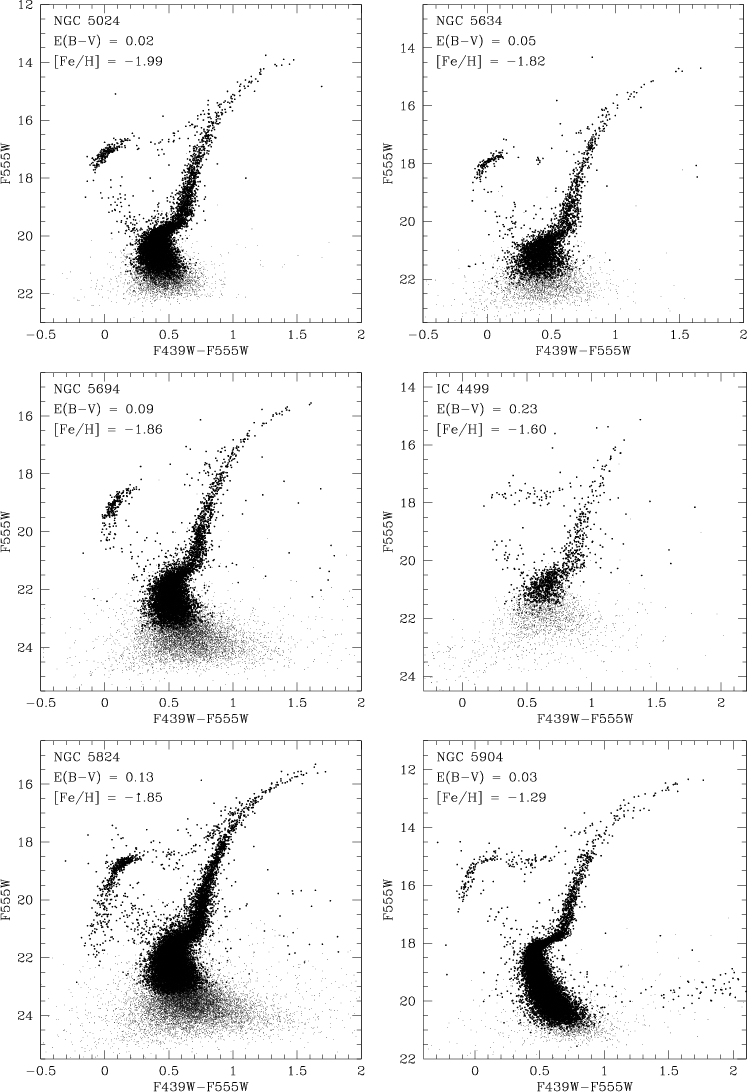
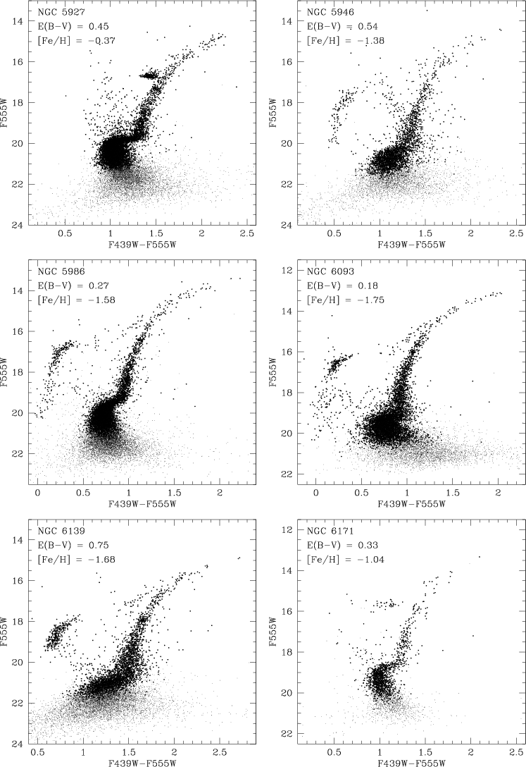
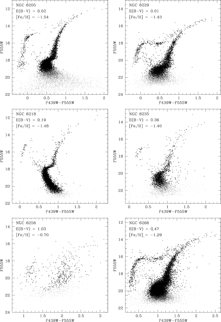
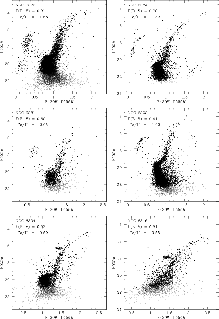
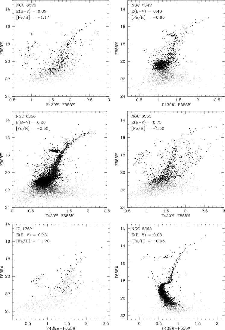
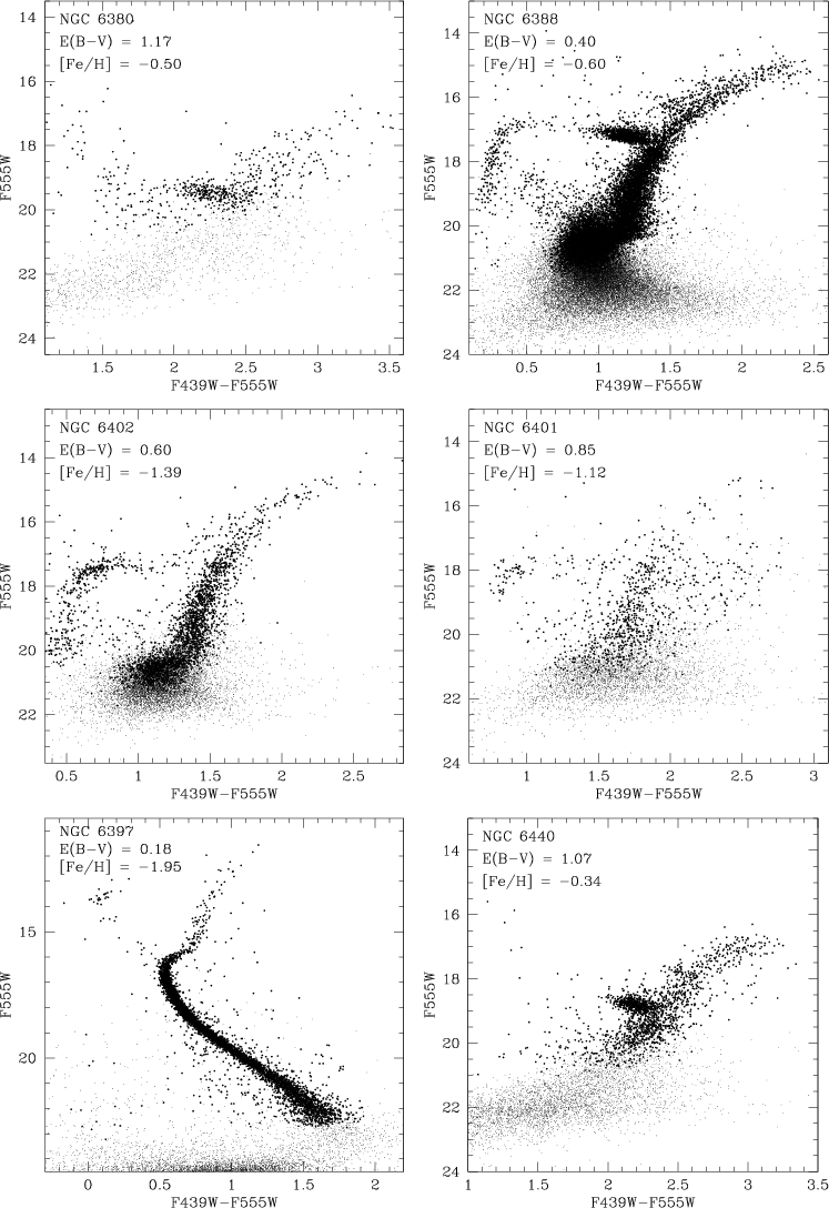
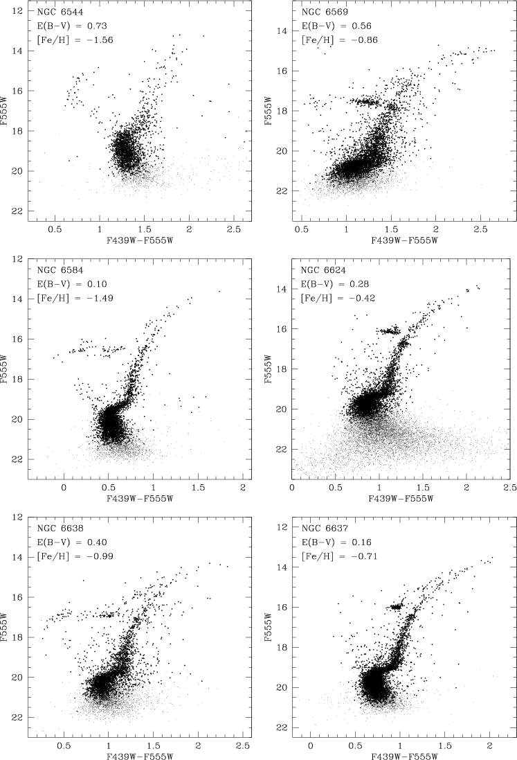
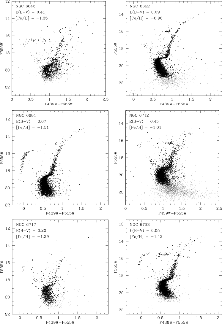
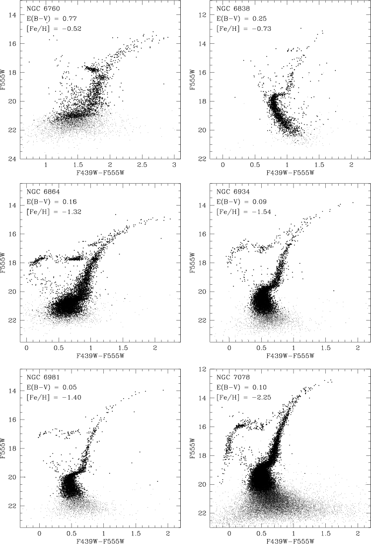
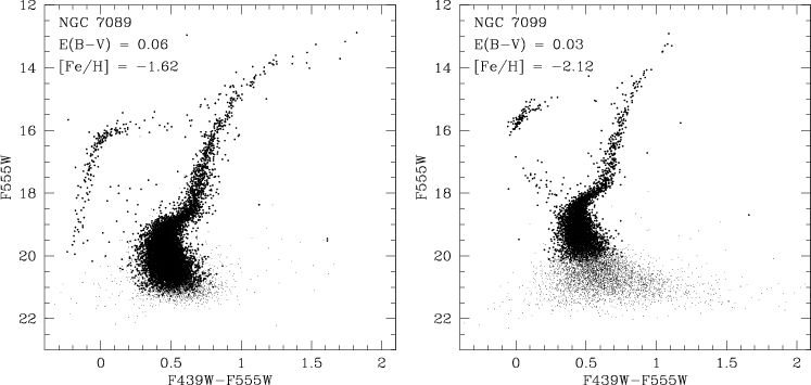
All the photometric data for the 74 GGCs presented in this paper come from HST/WFPC2 observations in the F439W and F555W bands; in all cases, the PC camera was centered on the cluster center. Table 1 list the observed clusters (Col. 1), the origin of the observations (Col. 2), and the exposure times in F555W (Col. 3) and F439W (Col. 4) bands. Table 2 give a few relevant parameters (from the Harris 1996 compilation) Fig. 1 shows the spatial distribution of the target clusters within the Galaxy.

Figure 1: Spatial distribution of the target clusters within the Galaxy.

After the snapshot observations (or, for 12 clusters, after the public release date), the images were retrieved via ftp from the HST archive in Baltimore, and they were furtherly processed partially following the recipe in Silbermann et al. (1996). As in Silbermann et al., the vignetted pixels, and bad pixels and columns, were masked out using a vignetting frame created by P. B. Stetson, together with the appropriate data-quality file for each frame. However, we did not correct for the pixel area map, since this correction is included in the calibration process described below. Finally the single-chip frames were extracted from the 4-chip-stack files, and analyzed separately. Frames obtained both at gain = and at were available, so care was taken to adjust the various parameters to the applicable gain value for each image.

 

 

Table 2: Main parameters of the clusters: Cols. 1 and 2 give the cluster identification number and other commonly used cluster name, Cols. 3 and 4 the Galactic longitude and latitude (degrees), Col. 5 gives the distance from the Galactic center (kpc), assuming R₀=8.0 kpc, Col. 6 the foreground reddening, Col. 7 the apparent visual distance modulus, Col. 8 the absolute visual magnitude, Col. 9 the metallicity [Fe/H], Col. 10 the central concentration ( $c = \log(r_{\rm t}/r_{\rm c})$, a "c'' denotes a core-collapsed cluster), Col. 11 the logarithm of core relaxation time ($\log$ (years)), Col. 12 the logarithm of relaxation time at the half-mass radius ($\log$ (years)), Col. 13 the logarithm of central luminosity density ($L_\odot$ pc^-3 ).

ID	Name	l	b	$R_{\rm GC}$	E(B-V)	(m-M)V	$M_{V\rm t}$	[Fe/H]	c	$r_{\rm t}$	$\log t_{\rm c}$	$\log t_{\rm h}$	$\log \rho_0$
NGC 104	47 Tuc	305.90	-44.89	7.4	0.04	13.37	-9.42	-0.76	2.03	47.25	8.06	9.48	4.77
NGC 362		301.53	-46.25	9.3	0.05	14.80	-8.40	-1.16	1.94c:	16.11	7.76	8.92	4.70
NGC 1261		270.54	-52.13	18.2	0.01	16.10	-7.81	-1.35	1.27	7.28	8.74	9.20	2.96
NGC 1851		244.51	-35.04	16.7	0.02	15.47	-8.33	-1.22	2.32	11.70	6.98	8.85	5.32
NGC 1904	M 79	227.23	-29.35	18.8	0.01	15.59	-7.86	-1.57	1.72	8.34	7.78	9.10	4.00
NGC 2419		180.37	25.24	91.5	0.11	19.97	-9.58	-2.12	1.40	8.74	9.96	10.55	1.54
NGC 2808		282.19	-11.25	11.0	0.23	15.56	-9.36	-1.15	1.77	15.55	8.28	9.11	4.61
NGC 3201		277.23	8.64	9.0	0.21	14.24	-7.49	-1.58	1.30	28.45	8.81	9.23	2.69
NGC 4147		252.85	77.19	21.3	0.02	16.48	-6.16	-1.83	1.80	6.31	7.49	8.67	3.48
NGC 4372		300.99	-9.88	7.1	0.39	15.01	-7.77	-2.09	1.30	34.82	8.90	9.59	2.09
NGC 4590	M 68	299.63	36.05	10.1	0.05	15.19	-7.35	-2.06	1.64	30.34	8.67	9.29	2.54
NGC 4833		303.61	-8.01	6.9	0.33	14.92	-8.01	-1.79	1.25	17.85	8.71	9.34	3.06
NGC 5024	M 53	332.96	79.76	18.8	0.02	16.38	-8.77	-1.99	1.78	21.75	8.79	9.69	3.04
NGC 5634		342.21	49.26	21.9	0.05	17.22	-7.75	-1.82	1.60	8.36	8.61	9.28	3.12
NGC 5694		331.06	30.36	29.1	0.09	17.98	-7.81	-1.86	1.84	4.29	7.86	9.15	4.03
IC 4499		307.35	-20.47	15.7	0.23	17.09	-7.33	-1.60	1.11	12.35	9.37	9.66	1.49
NGC 5824		332.55	22.07	25.8	0.13	17.93	-8.84	-1.85	2.45	15.50	7.88	9.33	4.66
NGC 5904	M 5	3.86	46.80	6.2	0.03	14.46	-8.81	-1.29	1.83	28.40	8.26	9.53	3.91
NGC 5927		326.60	4.86	4.5	0.45	15.81	-7.80	-0.37	1.60	16.68	8.29	8.98	3.87
NGC 5946		327.58	4.19	7.4	0.54	17.21	-7.60	-1.38	2.50c	24.03	7.06	8.95	4.50
NGC 5986		337.02	13.27	4.8	0.27	15.94	-8.42	-1.58	1.22	10.52	8.94	9.23	3.30
NGC 6093	M 80	352.67	19.46	3.8	0.18	15.56	-8.23	-1.75	1.95	13.28	7.73	8.86	4.76
NGC 6139		342.37	6.94	3.6	0.75	17.35	-8.36	-1.68	1.80	8.52	7.56	9.04	4.66
NGC 6171	M 107	3.37	23.01	3.3	0.33	15.06	-7.13	-1.04	1.51	17.44	8.05	9.31	3.13
NGC 6205	M 13	59.01	40.91	8.7	0.02	14.48	-8.70	-1.54	1.51	25.18	8.80	9.30	3.33
NGC 6229		73.64	40.31	30.0	0.01	17.46	-8.07	-1.43	1.61	5.38	8.36	9.19	3.40
NGC 6218	M 12	15.72	26.31	4.5	0.19	14.02	-7.32	-1.48	1.39	17.60	8.10	9.02	3.23
NGC 6235		358.92	13.52	2.9	0.36	16.11	-6.14	-1.40	1.33	7.61	8.11	8.67	3.11
NGC 6256		347.79	3.31	2.1	1.03	17.31	-6.02	-0.70	2.50c	7.59	5.36	8.40	5.70
NGC 6266	M 62	353.58	7.32	1.7	0.47	15.64	-9.19	-1.29	1.70c:	8.97	7.64	9.19	5.14
NGC 6273	M 19	356.87	9.38	1.6	0.37	15.85	-9.08	-1.68	1.53	14.50	8.50	9.34	3.96
NGC 6284		358.35	9.94	6.9	0.28	16.70	-7.87	-1.32	2.50c	23.08	7.15	9.16	4.44
NGC 6287		0.13	11.02	1.7	0.60	16.51	-7.16	-2.05	1.60	10.51	7.85	8.66	3.85
NGC 6293		357.62	7.83	1.4	0.41	15.99	-7.77	-1.92	2.50c	14.23	6.24	8.91	5.22
NGC 6304		355.83	5.38	2.1	0.52	15.54	-7.32	-0.59	1.80	13.25	7.38	8.89	4.39
NGC 6316		357.18	5.76	3.2	0.51	16.78	-8.35	-0.55	1.55	5.93	7.72	9.00	4.21
NGC 6325		0.97	8.00	2.0	0.89	17.68	-7.35	-1.17	2.50c	9.49	5.94	8.92	5.40
NGC 6342		4.90	9.73	1.7	0.46	16.10	-6.44	-0.65	2.50c	14.86	6.09	8.66	4.77
NGC 6356		6.72	10.22	7.6	0.28	16.77	-8.52	-0.50	1.54	7.97	8.33	9.26	3.76
NGC 6355		359.58	5.43	1.0	0.75	16.62	-7.48	-1.50	2.50c	15.18	5.95	8.71	4.95
IC 1257		16.53	15.14	17.9	0.73	19.25	-6.15	-1.70
NGC 6362		325.55	-17.57	5.3	0.08	14.79	-7.06	-0.95	1.10	16.67	9.07	9.31	2.22
NGC 6380	Ton 1	350.18	-3.42	3.2	1.17	18.77	-7.46	-0.50	1.55c:	12.06	8.39	8.87	3.70
NGC 6388		345.56	-6.74	4.4	0.40	16.54	-9.82	-0.60	1.70	6.21	7.90	9.24	5.31
NGC 6402	M 14	21.32	14.81	3.9	0.60	16.61	-9.02	-1.39	1.60	33.24	9.07	9.36	3.30
NGC 6401		3.45	3.98	0.8	0.85	17.07	-7.62	-1.12	1.69	12.10	7.74	9.29	4.10
NGC 6397		338.17	-11.96	6.0	0.18	12.36	-6.63	-1.95	2.50c	15.81	4.90	8.46	5.68
NGC 6440		7.73	3.80	1.3	1.07	17.95	-8.75	-0.34	1.70	6.31	7.54	8.76	5.28
NGC 6441		353.53	-5.01	3.5	0.44	16.62	-9.47	-0.53	1.85	8.00	7.72	9.13	5.23
NGC 6453		355.72	-3.87	3.3	0.61	17.13	-7.05	-1.53	2.50c	21.50	6.87	8.36	4.72
NGC 6517		19.23	6.76	4.3	1.08	18.51	-8.28	-1.37	1.82	4.10	6.90	8.88	5.20
NGC 6522		1.02	-3.93	0.6	0.48	15.94	-7.67	-1.44	2.50c	16.44	6.32	8.90	5.31
NGC 6539		20.80	6.78	3.1	0.97	17.63	-8.30	-0.66	1.60	21.46	8.60	9.37	3.62
NGC 6540	Djorg 3	3.29	-3.31	4.4	0.60	14.68	-5.38	-1.20	2.50c	9.49	5.01	7.08	5.92
NGC 6544		5.84	-2.20	5.4	0.73	14.33	-6.56	-1.56	1.63c:	2.05	5.05	8.35	5.75
NGC 6569		0.48	-6.68	1.2	0.56	16.43	-7.88	-0.86	1.27	6.95	8.25	9.17	3.76

 

Table 2: continued.

ID	Name	l	b	$R_{\rm GC}$	E(B-V)	(m-M)V	$M_{V\rm t}$	[Fe/H]	c	$r_{\rm t}$	$\log t_{\rm c}$	$\log t_{\rm h}$	$\log \rho_0$
NGC 6584		342.14	-16.41	7.0	0.10	15.95	-7.68	-1.49	1.20	9.37	9.01	9.09	2.92
NGC 6624		2.79	-7.91	1.2	0.28	15.37	-7.50	-0.42	2.50c	20.55	6.62	8.74	5.25
NGC 6638		7.90	-7.15	1.6	0.40	15.85	-6.83	-0.99	1.40	6.63	7.93	8.51	4.05
NGC 6637	M 69	1.72	-10.27	1.6	0.16	15.16	-7.52	-0.71	1.39	8.35	8.15	8.79	3.81
NGC 6642		9.81	-6.44	1.6	0.41	15.70	-6.57	-1.35	1.99	10.07	6.94	8.49	4.72
NGC 6652		1.53	-11.38	2.4	0.09	15.19	-6.57	-0.96	1.80	4.48	6.66	8.55	4.54
NGC 6681	M 70	2.85	-12.51	2.1	0.07	14.98	-7.11	-1.51	2.50c	7.91	5.62	8.83	5.41
NGC 6712		25.35	-4.32	3.5	0.45	15.60	-7.50	-1.01	0.90	7.44	8.86	8.98	3.14
NGC 6717	Pal 9	12.88	-10.90	2.3	0.20	14.95	-5.67	-1.29	2.07c:	9.87	6.61	8.26	4.65
NGC 6723		0.07	-17.30	2.6	0.05	14.87	-7.86	-1.12	1.05	10.51	8.99	9.30	2.81
NGC 6760		36.11	-3.92	4.8	0.77	16.74	-7.86	-0.52	1.59	12.96	7.94	9.39	3.84
NGC 6838	M 71	56.74	-4.56	6.7	0.25	13.75	-5.56	-0.73	1.15	8.96	7.64	8.41	3.05
NGC 6864	M 75	20.30	-25.75	12.8	0.16	16.87	-8.35	-1.32	1.88	7.28	7.85	9.08	4.51
NGC 6934		52.10	-18.89	14.3	0.09	16.48	-7.65	-1.54	1.53	8.37	8.43	9.07	3.37
NGC 6981	M 72	35.16	-32.68	12.9	0.05	16.31	-7.04	-1.40	1.23	9.15	8.93	9.20	2.35
NGC 7078	M 15	65.01	-27.31	10.4	0.10	15.37	-9.17	-2.25	2.50c	21.50	7.02	9.35	5.38
NGC 7089	M 2	53.38	-35.78	10.4	0.06	15.49	-9.02	-1.62	1.80	21.45	8.54	9.32	3.90
NGC 7099	M 30	27.18	-46.83	7.1	0.03	14.62	-7.43	-2.12	2.50c	18.34	6.38	8.95	5.04

2.2 Instrumental magnitudes

The photometric reduction was carried out using the DAOPHOTII/ALLFRAME package (Stetson 1987, 1994). Preliminary photometry was carried out in order to construct an approximate list of stars for each single frame. This list was used to match the different frames accurately. With the correct coordinate transformations among the frames, we obtained a single image, combining all the frames, regardless of the filter. In this way we could eliminate all the cosmic rays and obtain the highest signal/noise image for star finding. We ran the DAOPHOT/FIND routine on the stacked image and performed PSF-fitting photometry in order to obtain the deepest list of stellar objects free from spurious detections. The subtracted image was searched again for objects missed in the first pass, and the new list was appended to the existing one. Finally, the entire star list was given as input to ALLFRAME, for the simultaneous PSF-fitting photometry of all the individual frames. In some cases we could not construct a PSF from our images, since there were not enough sufficiently isolated stars in any of the four chips. In those instances, the PSFs used were the high-S/N PSFs extracted by P. B. Stetson (private communication) from a large set of uncrowded and unsaturated WFPC2 images. The clusters for which Stetson PSFs have been used are marked with an asterisk in Table 1. For each of the WFPC2 chips, the (typically two) F555W and (typically three) F439W magnitude lists were combined to create a raw color-magnitude diagram (CMD). First a catalog of mean magnitudes was created for each of the two filters, and then they were combined to obtain the F439W-F555W colors. In this process, we used the programs DAOMATCH/DAOMASTER (kindly provided by P. B. Stetson), which yield magnitudes in the instrumental photometric system of the two F555W and F439W frames that were chosen as references.

2.3 The correction for CTE

In order to calibrate our photometry, we followed the procedure outlined in Dolphin (2000; D00). This accounts for both the charge transfer (in)efficiency (CTE) and the variation of the effective pixel area across the WFPC2 field of view, and it yields final calibrated magnitudes in either the Johnson photometric system or the HST one. As a first step, a softened background was calculated from the actual output of ALLFRAME (after multiplying by the gain value G=7 or 15, so counts are expressed in electrons) as follows. Negative values of the background were set to zero, and then the background counts (B) were replaced by . The counts in electrons 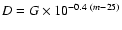were then computed for each star magnitude. (Note that DAOPHOT sets a star magnitude to m=25 for stars with a flux corresponding to one count above the sky background.) The B and D values were then used to find the CTE (and pixel area) correction to magnitude m, which is computed as m=m-C, where C=Y+X and

$$\begin{eqnarray*}X&=&\frac{x}{800}(0.024+0.002~\rm yr) \exp{[-0.196(\ln D-7)-0.1... ....507(\ln D-7)]}) \exp{[-0.035(\ln B-1)-0.042\cdot B]}\big\}\cdot \end{eqnarray*}$$

The CTE correction depends on the epoch of the observations (yr), which is expressed, in the D00 equations, relative to the reference epoch 1996.3. The coefficients of the equations were taken from Table 1 of D00, which is appropriate for observations made after April 23, 1994, when the camera was cooled from -76 $^{\circ }$C to -88 $^{\circ }$C. The corrected magnitudes were then calibrated to both the Johnson and HST flight systems, going through the steps described in the following Section.

2.4 Transformation to the standard photometric systems

The first step was to find the aperture corrections from ALLFRAME magnitudes to the reference aperture of 0.5'' used by Holtzman et al. (1995; H95). A set of bright isolated objects was selected, all their neighbors were subtracted, and aperture photometry was performed within the chosen set of radii. The aperture corrections were then defined as 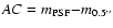, and median values were computed. Generally the agreement between the zero points of the four chips is good (  mag), but in some cases the procedure gave poor aperture corrections. This normally happened for the more crowded PC chip. In such cases, the aperture corrections were changed by a few hundredths of a magnitude in order to bring the PC photometry into agreement with the WF zero points. This procedure will of course erase any true magnitude offset introduced by a patchy reddening on arcmin scales, so we warn the readers that these data are not suitable for mapping the reddening within the sky area covered by the WFPC2.

Once the aperture corrections had been applied, the following procedure was followed. First, the aperture corrections AC₅₅₅ and AC₄₃₉, and the absorptions A₅₅₅ and A₄₃₉ were subtracted from the instrumental magnitues. Since the absorptions depend on the true colors, which are not known at the beginning, we started with null values for A₅₅₅ and A₄₃₉. From the corrected instrumental magnitudes m₅₅₅ and m₄₃₉ the counts were computed in the usual way, i.e., D₅₅₅=10^{-0.4(m₅₅₅-25)} and D₄₃₉=10^{-0.4(m₄₃₉-25)}. The D values were used to compute the provisional flight magnitudes, as given by the D00 equations:

$$\begin{array}{l} F555W=-2.5\log (D_{555}/t_{555})+21.734+\Del... ...\log (D_{439}/t_{439})+20.086+\Delta Z_{\rm CG}.\\ \end{array}$$

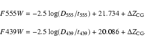
In these equations, t₅₅₅ and t₄₃₉ are the exposure times in seconds, the filter- and temperature-dependent zero-points were taken from Table 6 of D00 (Cold $Z_{\rm FG}$ column), and the chip to chip zero-point differences were in turn taken from Table 5. Explicitly, for gain 7 the values are 0.701, 0.761, 0.749, and 0.722 for the PC, WF2, WF3 and WF4 chips, respectively. For gain 15 the values are, in the same order of chips, -0.044, 0.007, -0.007, and -0.005.

The determination of the Johnson B and V magnitudes is complicated by the fact that they depend on the true color of the star, so we followed an iterative procedure. Assuming B-V=1, we computed the provisional magnitudes as prescribed by D00:

$$\begin{array}{l} V=F555W-0.060\times (B-V)+0.033\times (B-V)^... ...B=F439W+0.003\times (B-V)-0.088\times (B-V)^{2}.\\ \end{array}$$

We then computed an updated value of B-V and iterated until the difference between successive values of the magnitudes dropped below 0.001.

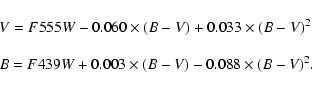
At this stage we are still ignoring absorption. However, we now have an estimate of the Johnson magnitudes, so we can compute a first provisional value of A₅₅₅ and A₄₃₉. They can be subtracted, together with the aperture corrections, from the instrumental magnitudes, and the previous cycle can be repeated until new values for the absorptions are obtained. Indeed, the cycle was repeated until again the differences between successive values of V and B were smaller than 0.001.

The absorptions were computed in the following manner. The absorptions for two stars of spectral type K5 and O6 are given in H95 for the different HST filters, as a function of the reddening E_B-V. In order to compute the absorption for a star of any spectral type, two fiducial B-V colors were assigned to the two reference types, B-V=1.15 and B-V=-0.32, respectively. The absorptions for stars of intermediate colors were computed as linear interpolations between the values at the two color extremes. Since the range in color of our stellar populations is not extreme, the same linear interpolation was used also to compute the absorptions for stars falling outside the preferred color range. The average reddening of each globular cluster was taken from the Harris (1996) catalog.

 

 

Table 3: Example of a photometry file (NGC 104, 47 Tuc): Col. 1 gives a star identification number, Cols. 2 and 3 give the position on the chip, Cols. 4 and 5 the V and B standard magnitudes (reddening corrected), Cols. 6 and 7 the F555W and F439W magnitudes in the HST flight system (reddening corrected), Cols. 8 and 9 the photometric errors given by ALLFRAME, Cols. 10 and 11 the V and Bstandard magnitudes (before the reddening correction), Cols. 12 and 13 the F555W and F439W flight magnitudes (before the reddening correction), Cols. 14 and 15 the $\chi$ and sharp parameters as given by ALLFRAME, and Col. 16 the chip number (1 for PC, and 2, 3, 4 for WF2, WF3, WF4 respectively).

ID	x	y	V	B	F555W	F439W	$\sigma_{F555W}$	$\sigma_{F439W}$
4	506.598	59.980	17.97	18.74	18.00	18.79	0.10	0.10
7	200.220	60.927	18.94	19.28	18.96	19.29	0.24	0.08
8	235.644	61.244	16.49	17.15	16.52	17.19	0.15	0.07
9	545.239	61.390	14.68	15.62	14.70	15.70	0.08	0.04
5	688.846	61.697	21.49	21.90	21.51	21.91	0.26	0.43
15	736.285	61.745	19.66	20.30	19.68	20.34	0.15	0.10
5603	537.317	62.062	18.96	19.48	18.99	19.50	0.16	0.08
12	445.775	62.208	18.65	19.37	18.67	19.42	0.09	0.06
14	636.699	62.301	18.00	18.65	18.02	18.69	0.08	0.06
11	119.039	62.725	17.59	18.03	17.61	18.04	0.09	0.06

$V_{\rm nr}$	$B_{\rm nr}$	$F555W_{\rm nr}$	$F439W_{\rm nr}$	$\chi$	sharp	chip
18.13	18.94	18.16	19.00	2.206	0.046	1
19.09	19.49	19.11	19.50	1.821	-0.032	1
16.65	17.35	16.67	17.39	6.213	0.157	1
14.83	15.82	14.86	15.90	9.128	0.040	1
21.64	22.10	21.66	22.12	1.015	-0.282	1
19.81	20.51	19.84	20.55	1.421	-0.041	1
19.12	19.68	19.14	19.71	2.239	0.162	1
18.80	19.57	18.83	19.62	1.677	0.079	1
18.15	18.85	18.18	18.90	2.230	0.108	1
17.75	18.23	17.77	18.25	1.887	-0.032	1

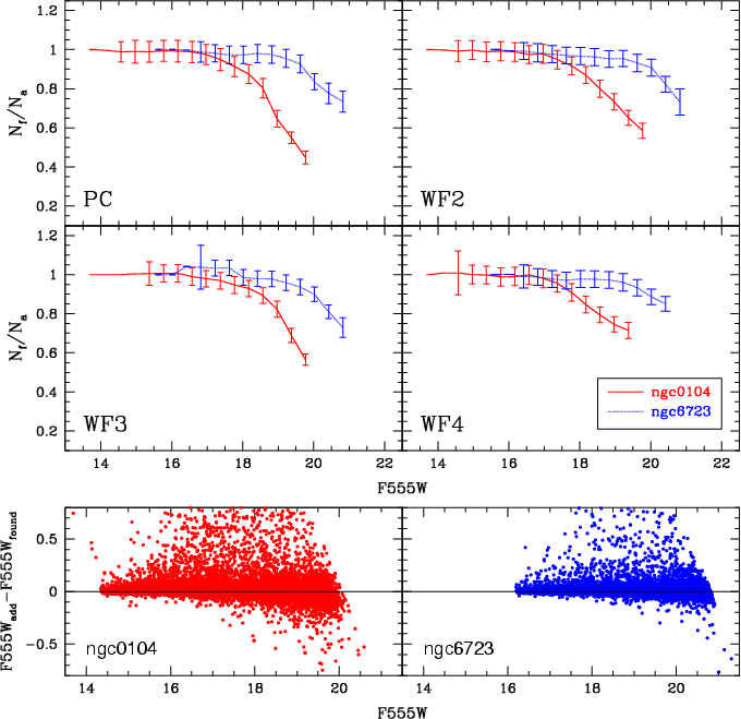Figure 2: Completeness functions and internal photometric errors from the artificial star experiments for the case of a high central density cluster (NGC 104), and of a low density object (NGC 6723).

In practice, it is impossible to directly compare the photometry of the data base published in this paper with any photometric catalog from groundbased data. Our HST images are on the central, very crowded regions which are not the usual targets of groundbased investigations. An indirect check of the photometric calibration is shown in Fig. 3, where the HB magnitude levels of the HST CMDs and of the CMDs from two groundbased photometric datasets are compared. The (upper panel) shows the differences between the V magnitudes of the horizontal branch ( ) of Rosenberg et al. (1999) and the for a subsample of our clusters (De Angeli 2001; Piotto et al. 2002), as a function of the reddening. In the lower panel, our  are compared with the corresponding values tabulated by Harris (1996). The for the HST data have been derived as in Zoccali et al. (1999). There is a good agreement between the HST and groundbased values.

2.5 Artificial star experiments and completeness

In order to correct the empirical star counts for completeness, we performed standard artificial star experiments for each GGC. In order to optimize the cpu time, in our experiments we tried to add the largest possible number of artificial stars in a single test, without artificially increasing the crowding of the original field, i.e., avoiding the overlap of two or more artificial-star profiles. To this purpose, as described in Piotto & Zoccali (1999), the artificial stars were added in a spatial grid such that the separation of the centers in each star pair was two PSF radii plus one pixel. The relative position of each star was fixed within the grid. However, the grid was randomly moved on the frame for each different experiment.

For each artificial star test, the frame-to-frame coordinate transformations (as calculated from the original photometry) were used to ensure that the artificial stars were added exactly in the same position in each frame. We started by adding stars in one Vframe at random magnitudes; the corresponding B magnitude for each star was chosen according to the fiducial points representing the instrumental CMD. The frames obtained in this way were processed following the same procedure used for the reduction of the original images.

The completeness fraction, typically in 0.4 mag intervals, was then computed as the ratio between the number of the added artificial stars and the number of artificial stars found in the same magnitude range.

We performed separate experiments for the HB, the subgiant and red giant branches, and the blue stragglers and main sequence. In each of the three CMD branches, we ran 8 independent experiments for each of the 4 WFPC2 chips, adding in each experiment 600 stars in the PC camera and 700 stars in the WF camera, for a total of more than 7100 experiments, with more than 5 million artificial stars added.

A comparison between the added magnitudes and the measured magnitudes allows us also a realistic estimate of the internal photometric error, defined as the standard deviation of the differences between the magnitudes added and those found, as a function of magnitude.

An example of the completeness functions, and of the internal photometric errors obtained from the artificial star experiments is shown in Fig. 2. We have selected two typical situations: (a) the case of a high central density cluster (NGC 104), and (b) the case of a low density object (NGC 6723).

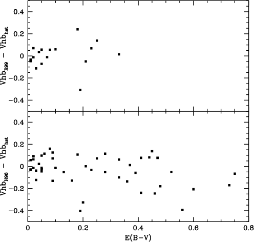Figure 3:   Upper panel: differences between the magnitude level of the HB ( ) of Rosenberg et al. (1999) and the for a subsample of our clusters (De Angeli 2001; Piotto et al. 2002) as a function of reddening. Lower panel: differences between the of Harris (1996) and the of a subsample of our clusters.

Figure 4: The F555W vs. F439W-F555W (flight system) color magnitude diagrams from the combination of the 4 WFPC2 cameras of 2 clusters of the database. Note that the magnitude and color ranges covered by each figure are always of the same size (though magnitude and color intervals start at different values). Heavier dots correspond to stars with an internal total error less than 0.1 mag.

Figure 4: continued.

Figure 4: continued.

Figure 4: continued.

Figure 4: continued

Figure 4: continued.

Figure 4: continued

Figure 4: continued.

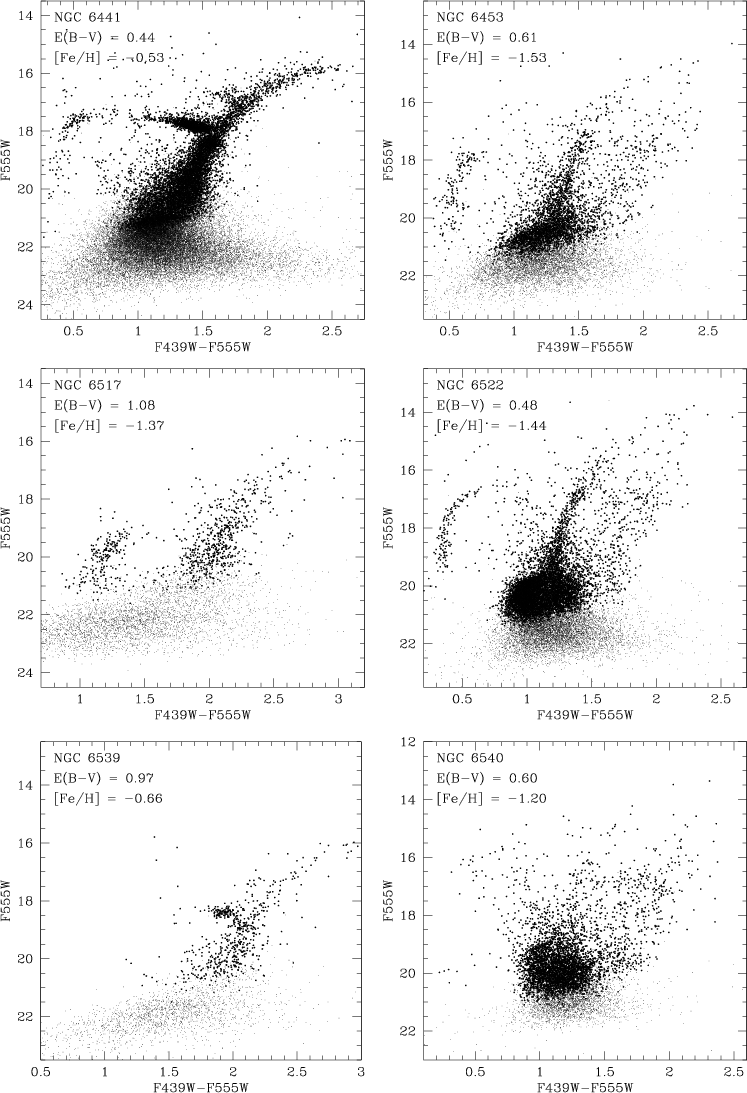Figure 4: continued. Note that the magnitude range of the CMD for NGC 6397 differs from the other cases.

Figure 4: continued.

Figure 4: continued.

Figure 4: continued.

Figure 4: continued.