5 Data reductions

The basic steps of the data reduction method are illustrated in Fig. 1. The successive steps, represented by boxes in the diagram, are explained in the following subsections.

The shaded box in Fig. 1 contains steps that are performed by the ELODIE software TACOS (Queloz 1996). Using the most recent Th-Ar exposure, TACOS computes a two dimensional Chebychev polynomial which maps each pixel to a wavelength. Using this map, the two-dimensional échelle spectrum is reduced to one-dimensional spectra on a nominal wavelength scale which therefore is based on the previous Th-Ar spectrum.

After resampling and conditioning (Sect. 5.1) the spectrum is digitally correlated with a synthetic template (Sect. 5.2), giving the spectral shift relative to the nominal wavelength scale. This is then corrected for short-term drift (Sect. 5.3), barycentric motion (Sect. 5.4) and long-term drift (Sect. 5.5). In this part of the reductions, shown by the upper branch in Fig. 1, all spectra receive exactly the same treatment, resulting in our estimated radial-velocity measures. For the lunar spectra it gives the radial-velocity measure of the Sun. In the lower branch of the diagram, used only for the spectra of the Moon, long-term drift (or the absolute zero point) is determined through cross-correlation with the Solar Flux Atlas (Kurucz et al. 1984); this defines the final wavelength scale.

The ELODIE software also provides radial-velocity determinations based on either or both of two standard ELODIE templates, corresponding to F0V and K0III stars (both containing box-shaped lines derived from model atmosphere spectra, see Baranne et al. 1996). These velocities are not further discussed in this paper, although they did provide a useful consistency check of our own procedure.

   
5.1 Resampling and conditioning of the spectrum

Before correlating, all 67 orders extracted by the ELODIE software are combined into a single one-dimensional spectrum, normalised, flipped, resampled and windowed. This conditioning of the spectrum is illustrated in Fig. 2.

The purpose of the normalisation is to equalise the flux distribution, so that the relative weights of different spectral regions is independent of arbitrary factors such as the wavelength response of the spectrometer (cf. Sect. 7.3). Tungsten exposures are used to remove the main part of the variation within each order. "Continuum'' points are then identified and used to normalise the flux values to the interval [0,1]. Data from the different orders are combined into a single sequence of flux/wavelength pairs by removing the blue ends of overlapping orders.

Both the observed data set and the template are then flipped and resampled with a constant step of $\Delta\Lambda=5\times 10^{-7}$ in $\Lambda=\ln\lambda$. Using a logarithmic wavelength scale renders the Doppler shift independent of wavelength (cf. Sect. 3). The chosen resampling step, corresponding to a velocity step of $\simeq$150 m s^-1, is more than adequate to preserve all spectral information (it gives $\simeq$50 steps across the instrumental FWHM, and $\simeq$20 steps per pixel), and allows accurate sub-step centroiding by simple interpolation (Eq. (5)). The resulting resampled data sequence is denoted $(\Lambda_i,f_i)$, $i=1\dots n$. To avoid spurious effects from the edges of the stellar spectrum and template, the flux data are furthermore multiplied with a flat-topped cosine window function $0\le w_i \le 1$, such that the outermost 5% at each end smoothly taper off to zero.

   
5.2 Digital cross-correlation

The ELODIE radial-velocity measurements are normally based on synthetic templates derived from stellar atmosphere models. We have instead chosen to use a template based only on 1340 Fe I lines, for which very accurate laboratory wavelengths exist (Nave et al. 1994). The lines were selected in the wavelength region 400-680 nm through comparison with the Allende Prieto & García López (1998a) catalogue of solar lines. The majority of the lines are of quality grade `A' in the list by Nave et al.  implying wavenumber uncertainties below 0.005 cm^-1 or 75 m s^-1 at $\lambda=500$ nm, and have upper levels of moderate excitation (<6.5 eV), for which pressure-dependent shifts in the laboratory wavelengths should be small. The template was built by unit height Gaussian functions having a constant FWHM of W=5 km s^-1. For the lunar observations, we also use the Solar Flux Atlas (Kurucz et al. 1984) as template.

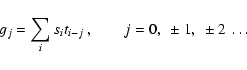
Let s_i=w_i f_i, $i=1\dots n$ be the stellar spectrum resulting from the conditioning described above, and t_i the similarly conditioned template. Both data sets are equidistantly sampled in $\Lambda=\ln\lambda$ with step $\Delta\Lambda$. The cross-correlation function (CCF) is computed as

$$g_j = \sum_i s_i t_{i-j}~ ,\qquad j=0,~\pm 1,~\pm 2~\dots$$ (4)

These values can be regarded as discrete points of the continuous CCF g(u) for $u=j\Delta\Lambda$. The cross-correlation process should find $\hat{u}$ such that $g(\hat{u})$ is the global maximum of the CCF. We do this by fitting a parabola to the three points nearest to the maximum of the discrete CCF and computing the point where the analytical derivative of the parabola is zero (g'(u)=0). If g_jis the highest point in the discrete CCF ( $g_{j-1} \le g_j > g_{j+1}$), then

$$\hat{u} = \left[ j + \frac{\frac{1}{2} (g_{j+1}-g_{j-1})}{2g_j-g_{j-1}-g_{j+1}}\right] \Delta\Lambda ~ .$$ (5)

Multiplying $\hat{u}$ with the speed of light gives the shift $d_{\rm N}$expressed in velocity units. The subscript "N'' indicates the nominal wavelength scale obtained from the current Th-Ar calibration.

The uncertainty of $\hat{u}$ from photon and readout noise in the CCD image, $\sigma_{\hat{u}}$, is estimated according to Eq. (A.3) derived in the appendix. In velocity units $\sigma_{\rm N}=c\sigma_{\hat{u}}$ranges from 2 m s^-1 to several 100 m s^-1 for the observations reported in Table 2; the median value is 13 m s^-1.

A short remark should be made concerning our method to compute the maximum of the digital CCF. An alternative procedure described in the literature (e.g. Murdoch & Hearnshaw 1991; Gunn et al. 1996; Skuljan et al. 2000) is to fit a Gaussian, or some other suitable function, to a wider part of the correlation peak. We believe that this procedure is inappropriate from the viewpoint of statistical estimation theory in our case, or when model-atmosphere spectra are used as templates. Maximising the CCF is equivalent to minimising the $\chi^2$ or some similar function representing the goodness-of-fit between the template and spectrum, and it is then the extreme point of the objective function that should be sought.

Figure 3: The left panels show the drift of the Th-Ar calibration for observations made in February 1997; the right panels show the corresponding data for October 1997. The upper panels show the accumulated drift during the nights from an arbitrary origin. The lower panels show the drift between successive Th-Ar calibration exposures as function of the time interval between them.

Figure 4: This plot is similar to the lower panels in Fig. 3, except that more points are added representing all possible data pairs $(\Delta t,\Delta v)$ (i.e. not just successive exposures). The thick dots show a moving average using a window of 0.5 hour. The continuous curves show the fitted function $\Delta v_{\rm rms}=(a+b\Delta t)^{1/2}$ representing a Wiener process plus white noise.

   
5.3 Short-term drift correction

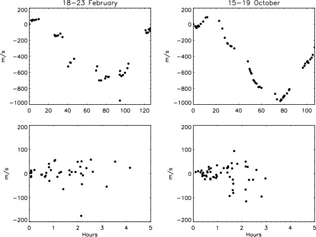
Short-term stability of the ELODIE spectrometer is normally ensured by recording a Th-Ar exposure simultaneously with the stellar spectrum. In our case the calibration (Th-Ar) exposures were temporally separated from the stellar or lunar observations, and a small correction for the short-term drift was therefore necessary. The drift in velocity from one calibration exposure to the next is readily derived from the logged data, and allow to reconstruct the drift as function of time from an arbitrary origin (top panels of Fig. 3). Within each night the drift is reasonably smooth, especially in the October data, which makes it meaningful to derive corrections through linear interpolation between successive calibration exposures.

To estimate the uncertainty of such corrections, a statistical model of the drift is needed. The lower panels of Fig. 3 show how the drift ($\Delta v$) statistically increases with the time interval ($\Delta t$) between successive exposures. In Fig. 4 the absolute drift values $\vert\Delta v\vert$ are shown for all pairs of calibration exposures, together with running averages. We adopt the drift model ${E}(\Delta v^2)=a+b\Delta t$, i.e. a Wiener (random-walk) process (e.g. Grimmett & Stirzaker 1982) plus a white-noise term (a) accounting for uncorrelated measurement noise. The fitted curves in Fig. 4 are for

$$\left. \begin{array}{lll} a=170~\mbox{m}^2~\mbox{s}^{-2}~ ... ...{s}^{-3} &\quad \mbox{(October)} \\ \end{array}\right\}\cdot$$ (6)

Let $\Delta v_1$ (at time t₁) and $\Delta v_2$ (at t₂) be two successive drift measurements. The interpolated drift at the intermediate time t is $\Delta v=(1-f)\Delta v_1 + f\Delta v_2$, where f=(t-t₁)/(t₂-t₁). (Actually, the correction applied is the drift since the previous Th-Ar calibration exposure, $d_{\rm D}=\Delta v -\Delta v_1$.) The uncertainty of the correction is

$$\sigma_{\rm D}=\sqrt{\left[{\textstyle\frac{1}{2}}- f(1-f)\right]a+f(1-f)(t_2-t_1)b} ~ .$$ (7)

A few stellar observations were made after the last Th-Ar exposure of the night, in which case no short-term drift correction was applied. The resulting uncertainty is

$$\sigma_{\rm D}=\sqrt{{\textstyle\frac{1}{2}}a+(t-t_1)b} ~ .$$ (8)

Although the data suggest a much improved instrument stability in the October period, we use the more conservative values a=170 m² s^-2, b=0.19 m² s^-3 to estimate the drift uncertainty in both observation periods. With intervals up to 3.5 hr between calibration exposures, the uncertainty of the drift correction could in some cases amount to 25 m s^-1. The median $\sigma_{\rm D}$ is 17 m s^-1.

 

 

Table 1: Observations of the Moon, from which the long-term drift correction is determined, and subsequently the barycentric radial-velocity measure of the Sun. The columns contain: Date - mean epoch of observation, given as the topocentric Julian Ephemeris Date (JED) minus 2450000.0; $d_{\rm N}~({\rm SFA})$ - nominal spectral shift obtained by correlating with the Solar Flux Atlas (Kurucz et al. 1984); $d_{\rm D}$ - short-term drift correction; $v_{\rm LOS}$ - line-of-sight velocity (Sun-Moon-observer light path); $d_{\rm B}$ - resulting barycentric shift with respect to the Solar Flux Atlas; $d_{\rm N}~({\rm Fe {\sc i}})$ - nominal shift obtained by correlating with the synthetic Fe I template; d₀ - long-term drift correction (mean value of $-d_{\rm B}$); $cz_{\rm B}$ - barycentric radial-velocity measure of the Sun (referring to the Fe I template), including the correction from Eq. (2); mean value and dispersion of the barycentric radial-velocity measures for the 1997 February and October observation periods. Indicated uncertainties are internal standard errors.

Date	$d_{\rm N}(\mbox{SFA})$	$d_{\rm D}$	$v_{\rm LOS}$	$d_{\rm B}$		$d_{\rm N}(\mbox{Fe {\sc i}})$	d0	$cz_{\rm B}$	mean value
2450000+	km s-1	km s-1	km s-1	km s-1		km s-1	km s-1	km s-1	km s-1
498.2761	+0.688	-0.003	-0.785	-0.100$~\pm~$0.018		+0.960	+0.090	+0.267$~\pm~$0.018
498.2819	+0.704	-0.007	-0.794	-0.097$~\pm~$0.021		+0.978	+0.090	+0.272$~\pm~$0.021
498.2854	+0.724	-0.009	-0.799	-0.084$~\pm~$0.023		+0.999	+0.090	+0.286$~\pm~$0.023	+0.277$~\pm~$0.010 (Feb.)
498.2899	+0.720	-0.011	-0.806	-0.097$~\pm~$0.024		+0.992	+0.090	+0.270$~\pm~$0.024
498.2927	+0.749	-0.013	-0.810	-0.074$~\pm~$0.026		+1.021	+0.090	+0.293$~\pm~$0.026
737.3799	-0.537	-0.002	+0.556	+0.017$~\pm~$0.011		-0.302	-0.016	+0.240$~\pm~$0.011
737.3841	-0.518	-0.002	+0.550	+0.030$~\pm~$0.013		-0.284	-0.016	+0.252$~\pm~$0.013
737.3910	-0.520	-0.002	+0.539	+0.017$~\pm~$0.009		-0.286	-0.016	+0.240$~\pm~$0.009
740.4709	-1.152	-0.001	+1.163	+0.010$~\pm~$0.010		-0.921	-0.016	+0.229$~\pm~$0.010	+0.238$~\pm~$0.008 (Oct.)
740.4750	-1.151	-0.001	+1.158	+0.006$~\pm~$0.011		-0.917	-0.016	+0.228$~\pm~$0.011
740.4778	-1.133	-0.002	+1.154	+0.019$~\pm~$0.013		-0.897	-0.016	+0.243$~\pm~$0.013
740.4806	-1.133	-0.003	+1.150	+0.014$~\pm~$0.013		-0.902	-0.016	+0.233$~\pm~$0.013

   
5.4 Barycentric correction

For the observations of stars, the barycentric correction amounts to the application of the two factors in Eq. (1). $v_{\rm LOS}$ is provided by the ELODIE software for the effective (i.e., flux-weighted) mean time of observation (Baranne et al. 1996). However, in a few cases the timing automatically logged by the ELODIE system was clearly offset, and we therefore chose to re-compute this velocity for all the observations. The mean epoch of observation was reconstructed from the observers' notes, and the barycentric velocity of the observatory $\vec{v}_{\rm obs}$ obtained from JPL's Horizons On-Line Ephemeris System (Giorgini et al. 1996; Chamberlin et al. 1997). For the same epoch, the coordinate direction $\vec{k}$ to the star was computed using data from the Hipparcos Catalogue (Turon et al. 1998). Both vectors are expressed in the ICRF frame, so $v_{\rm LOS}=\vec{k}{'}\vec{v}_{\rm obs}$ follows as the scalar product. In the mean, the values provided by the ELODIE software agreed well with our calculations, but in 7 cases (out of 76) the difference exceeded 10 m s^-1, and in 2 cases it exceeded 200 m s^-1.

For an observation spanning the time interval $[t_{\rm beg},t_{\rm end}]$the barycentric correction used $v_{\rm LOS}(t_{\rm mid})$ computed for the exposure mid-time, $t_{\rm mid}=(t_{\rm beg}+t_{\rm end})/2$. There is an uncertainty in this correction due to the unknown difference between $t_{\rm mid}$ and the actual flux-weighted mean epoch of observation. We estimate this uncertainty to be around 10 per cent of the variation of the barycentric correction over the exposure, or $\sigma_{\rm LOS} = 0.1\times \vert v_{\rm LOS}(t_{\rm end})- v_{\rm LOS}(t_{\rm beg})\vert$. The median uncertainty per observation from this effect is 13 m s^-1.

The observations of the Moon, in the upper branch of Fig. 1, receive a corresponding barycentric correction, including the factor Eq. (2), only with $v_{\rm LOS}$ computed through numerical differentiation of the total path length from the Sun to the observer, $\left\vert\vec{r}_{\rm M}(t_{\rm M})-\vec{r}_\odot(t_\odot)\right\vert+ \left\vert\vec{r}_{\rm M}(t_{\rm M})\right\vert$. Here $\vec{r}_\odot(t)$and $\vec{r}_{\rm M}(t)$ are the geometric ephemerides of the Sun and the subterrestrial point on the Moon, respectively, relative the observer; $t_{\rm M}$ and $t_\odot$ are the time of observation diminished by the light time to the respective object. Relative geometric coordinates were obtained via the JPL Horizons system. In this calculation it was assumed that the telescope was pointed at the geometrical centre of the lunar disk. This is not a critical issue: a depointing by one tenth of the moon's apparent diameter would at most cause an error of 0.6 m s^-1 in the barycentric correction.

In the lower branch of Fig. 1 the observations are correlated with the Solar Flux Atlas (Kurucz et al. 1984), and the barycentric correction must here be defined as was done for the Atlas. From the description of the latter we infer that no correction corresponding to Eq. (2) was used in constructing its rest wavelength scale. Consequently, in the lower branch of Fig. 1, the barycentric correction amounts only to the factor $1+v_{\rm LOS}/c$.

   
5.5 Long-term drift correction (absolute zero point)

The long-term drift correction is computed on the assumption that the solar spectrum has no intrinsic long-term velocity variations and that the wavelength scale in the Solar Flux Atlas is correct. These assumptions are further discussed in Sect. 7.1.

The correlation of a Moon spectrum with the Solar Flux Atlas gives the shift $d_{\rm N}({\rm SFA})$ in the second column of Table 1. This is expressed on the nominal wavelength scale of the previous Th-Ar exposure. After correction for the short-term drift ($d_{\rm D}$) and line-of-sight velocity ( $v_{\rm LOS}$) we obtain the barycentric quantity $d_{\rm B}$, which should be zero if the Th-Ar wavelengths are effectively on the same scale as the wavelengths in the Solar Flux Atlas. As shown in the table, $d_{\rm B}$ is significantly different between the February and October sessions (while the variations within each session are hardly significant). As discussed in Sect. 7.1, it is likely that this difference is (mainly) an instrumental effect, perhaps resulting from some readjustment of the spectrometer made between the two observing sessions.

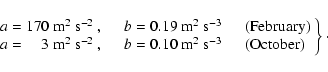
Accordingly, we adopt the mean $-d_{\rm B}$ in each observing period as the long-term drift correction, or absolute zero point (d₀) for the radial-velocity measures. This gives $d_0=+0.090\pm0.010$ km s^-1for the February data, and $d_0=-0.016\pm0.007$ km s^-1 for October. For both periods we adopt $\sigma_0=0.010$ km s^-1 as the zero-point uncertainty.

5.6 Combined corrections

The observed spectral shift, corrected for short-term drift and zero point, is given by

$$c\ln(1+z_{\rm obs}) = d_{\rm N}(Fe {\sc i}) + d_{\rm D} + d_0 ~ .$$ (9)

Inserting this in Eq. (1) and expanding exponentials to second order gives

$$cz_{\rm B} = D + \frac{1}{2c}\left( D^2 - v_{\rm LOS}^2 \right) ~ ,$$ (10)

where

$$D = d_{\rm N}(Fe {\sc i}) + d_{\rm D} + v_{\rm LOS} + d_0 + (4.44~\mbox{m~s}^{-1})$$ (11)

(this approximation should not be used for velocities above some 600 km s^-1, cf. Sect. 3).

The total internal error of $cz_{\rm B}$ is obtained as the sum in quadrature of the standard errors of the terms in Eq. (11), viz. $\sigma_{\rm N}=c\sigma_{\hat{u}}$ from Eq. (A.3), $\sigma_{\rm D}$ from Eq. (7) or (8), $\sigma_{\rm LOS}$ from Sect. 5.4, and $\sigma_0$ from Sect. 5.5. The error in the last term of Eq. (11) is neglected. In the cases where the final radial-velocity measure is computed as a mean of N>1 observations, $\sigma_0$ is applied after the averaging (thus $\sigma_0$ is not reduced by N^-1/2). Typical values of the errors are summarised in Table 3.

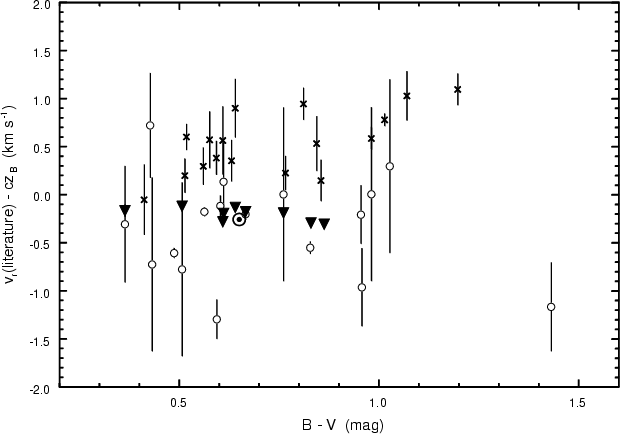Figure 5: Differences between various radial-velocity determinations in the literature ( $v_{\rm r}({\rm CDS})$ or $v_{\rm r}({\rm other})$ in Table 2) and our radial-velocity measures, plotted against colour index. Error bars show $\pm 1\sigma$, where $\sigma$ is the sum in quadrature of the uncertainties in Table 2. Only data with $\sigma <1$ km s-1are plotted. Crosses are for $v_{\rm r}$ by Griffin et al. (1988), filled triangles by Nidever et al. (2002), and open circles from other sources. For the Nidever et al. differences, the error bars are too small to be visible in the diagram. The solar symbol shows the difference for the Sun, knowing its $v_{\rm r}=0$.