3 Velocity field generation

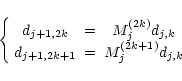
We generate a velocity field by constructing its wavelet decomposition coefficients. We use the concept of multi-resolution associated with an orthogonal wavelet (see Mallat 1999): the dilated and translated family

$$\left\{ \psi _{j,n}(t)=\frac{1}{\sqrt{2^{j}}}~ \psi \left( \frac{t-2^{j}k}{2^{j}}\right) \right\} _{(j,k)\in Z}$$ (6)

can be an orthonormal basis of L²(R) on which any function may be decomposed. With f the velocity field, we have:

 

$$\forall f\in L^{2}(\Re ),f \sum_{j}\sum_{k}<f,\psi_{j,k}>\psi_{j,k}$$ =

$$\sum_{j}\sum_{k}~ d_{j,k}~ \psi _{j,k}$$ = (7)

where $d_{j,k}=~<f,\psi _{j,k}>$ are the wavelet coefficients, but also for any j₀

$$f=\sum _{0\leq k<2^{j_{0}}}c_{j_{0},k~ }\phi _{j_{0},k}+\sum _{j\geq j_{0}}~ \sum _{0\leq k<2^{j}}d_{j,k}~ \psi _{j,k}$$ (8)

where $\phi _{j_{0},k}$ is the scaling function associated with $\psi$ (see Mallat 1999). The c_j0,k (approximation coefficients) and the d_j,k (detail coefficients) completely characterise f, and one still has the freedom to choose the scale threshold j₀ at which the field f is approximated. To build a velocity signal which has a resolution 2^-n, we set j₀=0, c_0,0=0 (which means that we are in the centre-of-mass frame), and d_j0,0 to a non-zero value. Then all the coefficients d_j+1,k are generated from the d_j,k by a multiplicative log-normal process with prescribed coefficients. Thus, we obtain a synthetic velocity field with the same statistical properties as the one analysed. More precisely the d_j,k are obtained by

$$\left\{ \begin{array}{ccc} d_{j+1,2k} & = & M^{(2k)}_{j}d_{j,k}\\ d_{j+1,2k+1} & = & M^{(2k+1)}_{j}d_{j,k} \end{array}\right.$$ (9)

where $\left\vert M^{(k)}_{j}\right\vert$ are realisations of a random variable M_j that follow the log-normal law from Sect. 2.2 with a=2^-j and  a'=2^-j-1. Numerical values of the velocity are expressed in units of d_j0,0.

The standard deviation of the velocity field as a function of size is plotted in Fig. 4. The law $\sigma _{l}(v)\propto l^{\beta}$ fits both the synthetic velocity field and the Polaris region well with an exponent of $\beta \simeq 0.5$ in both cases. This exponent is clearly irrelevant (or equal to 0) for a classical Gaussian field: for such a field the standard deviation is the same for any scale; the difference observed is just a sampling effect. The model is adjusted to observations by fixing d_0,0 so that the curves coincide. Here, d_0,0=250 for 13 octaves (reductions of scale by a factor of 2) between the integral scale and the $\Delta =2$ scale.

The resulting velocity field is then submitted to the same analysis as the original one, and the number of steps between our integral scale and the Polaris map scale is fixed by adjusting the non-Gaussian wings. Figure 5 shows the resulting PDFs. Here N=13between the integral scale and the $\Delta =2$ scale. Note that the synthetic field PDFs are in good agreement with the observed ones, and that the synthetic field is correlated at all scales (a rough estimate of the synthetic signal correlation length at scale ais a) unlike the uncorrelated Gaussian field used for comparisons.

We are now able to determine the scaling of our model by identifying size at scale N with Polaris resolution. In Fig. 5, $\Delta =2$ pixels corresponds to l_N=2250 AU, so that our integral scale is $l_{0}=2^{N}.2250~ {\rm AU}=90~{ \rm pc}$. Note that this is not the size of the cloud that we generate: the Polaris map size is reached after 9 steps in the generating process. A side effect of that sub-sampling is that the mean global velocity of the generated cloud is slightly non 0.0 (see Sect. 4.4).

Figure 4: Standard deviation of the velocity field as a function of size l (in pixel units) for Polaris, for the synthetic field, and for a Gaussian field. The vertical offset of the model is fixed by  . Straight lines are power laws with an exponent .

Figure 5: Comparison between the velocity increments' PDFs of the Polaris map (points) and the reconstructed field (lines) for different scales.