

Up: The co-orbital corotation torque
Appendix A: Finite resolution effects on the co-orbital corotation torque estimate
As the radial width of the co-orbital region in the simulations presented in this work amounts to a small number of
zone widths (typically 3 to 18),
it is of interest to investigate how bad or good is the code used here in giving an estimate of the
co-orbital corotation torque. For this purpose, one can consider a simplified situation, such as the one depicted at
Fig. A.1. This situation neglects the grid curvature and describes the gas flow around the planet in
a shearing sheet. In this situation, the corotation torque is given by
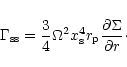 |
(A.1) |
![\begin{figure}
\par\includegraphics[width=8.7cm,clip]{resol1.eps}
\end{figure}](/articles/aa/full/2002/20/aa1942/Timg268.gif) |
Figure A.1:
Sketch of a shearing sheet case. A radial set of zones is represented. The
separatrices are assumed to be horizontal and are symmetric w.r.t. the orbit.
The azimuthal velocity is set on a staggered mesh (centered in radius,
staggered in azimuth), and is assumed in this simplified example to be
independent of azimuth. |
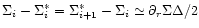
The code used here enforces angular momentum conservation (to the computer accuracy) hence the balance of angular
momentum gained/lost by the orbit crossing fluid elements on horseshoe streamlines can be used as an estimate of the
corotation torque. The angular momentum is a zone centered variable. In this simplified situation the velocity field is
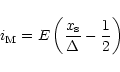
assumed to be the unperturbed one. The zone radial index is denoted i, and vanishes at the orbit (as stated in
Sect. 3, the planet lies in the center of a zone). The index of the outermost zone fully embedded in
the co-orbital region is denoted  .
It is assumed that the co-orbital region is wide enough so that such a zone exists. The
expression for
is therefore:
.
It is assumed that the co-orbital region is wide enough so that such a zone exists. The
expression for
is therefore:
 |
(A.2) |
where E(X) stands for the integer part of X, and where  is the radial zone width.
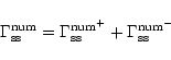
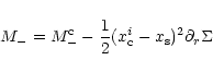
The co-orbital corotation torque in this situation can therefore be expressed as:
is the radial zone width.
The co-orbital corotation torque in this situation can therefore be expressed as:
 |
(A.3) |
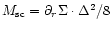
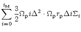
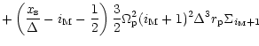
where:
is the torque due to the horseshoe fluid elements flowing from  to
to  ,
and where:
,
and where:
is the torque due to the horseshoe fluid elements flowing from  to .
If one writes:
to .
If one writes:
![\begin{displaymath}
\Sigma_i=\Sigma_0+i\Delta\frac{\partial\Sigma}{\partial r}+O[(i\Delta/r_{\rm p})^2]
\end{displaymath}](/articles/aa/full/2002/20/aa1942/img281.gif) |
(A.6) |
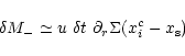
then combining Eqs. (A.4) and (A.5) one is led to:
The relative error on the corotation torque evaluation,
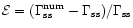 ,
is therefore given by:
,
is therefore given by:
![\begin{displaymath}
{\cal E}(Y) = \frac{4}{Y^4}\left[\sum_{i=0}^{i_{\rm M}}i^3+(i_{\rm M}+1)^3\left(Y-i_{\rm M}-\frac 12\right)\right]
\end{displaymath}](/articles/aa/full/2002/20/aa1942/img286.gif) |
(A.8) |
where
 is the horseshoe region half-width, expressed in zone radial widths. The graph of the function
 is the solid line of Fig. A.3.
The second step of this error estimate consists of evaluating the discrepancy between the actual and effective
separatrix position. Indeed, the brackets of the second line of Eqs. (A.4)
and (A.5) stand for the mass fraction of the outermost horseshoe zone included within the separatrix (i.e. it is
also the ratio of the shaded area surface to the zone
surface in Fig. A.1). There is no warranty however that the separatrix position which has to be used in this
evaluation coincides with the one provided by the streamline analysis. In other words, one has to evaluate how much
separatrix crossing numerical effects can lead to, in order to infer how distant the actual and effective separatrices can be.
One approximate way to do that is to consider a 1D problem (along the radial dimension). Disregarding azimuthal advection
should not lead to significant errors, as this latter is treated apart during the advection procedure based on the
operator splitting technique, and as azimuthal motion should not lead to separatrix crossing provided this latter is
horizontal (or weakly tilted) in the
 plane.
![\begin{figure}
\par\includegraphics[width=8.8cm,clip]{resol2.eps}
\end{figure}](/articles/aa/full/2002/20/aa1942/Timg289.gif) |
Figure A.2:
Sketch of the 1D mesh used to evaluate the impact of numerical effects on
separatrix crossing. The linear density  is zone-centered, while
the radial velocity u is defined at zone interfaces (on a staggered mesh).
is zone-centered, while
the radial velocity u is defined at zone interfaces (on a staggered mesh). |
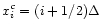
Following the notations of Fig. A.2, one can write the total mass M- contained below the separatrix (or
below any arbitrary position  )
at time t as:
)
at time t as:
 |
(A.9) |
where
is the zone spacing. This mass will be referred to hereafter as the
inner mass. At time
 ,
the inner mass becomes:
,
the inner mass becomes:
M-'= |
(A.10) |
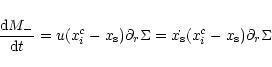
where the primes denote the new quantities, and where one has the following relationship:
 |
(A.11) |
where Fj is the mass flux (oriented upwards) across the interface between the zones j-1 and j. One also needs the
following relationship:
![\begin{displaymath}x_{\rm s}'=x_{\rm s}+\delta t\left[u_i\left(i+1-\frac{x_{\rm ...
...}\right)+u_{i+1}\left(\frac{x_{\rm s}}{\Delta}-i\right)\right]
\end{displaymath}](/articles/aa/full/2002/20/aa1942/img294.gif) |
(A.12) |
which comes from the fact that the streamlines (and therefore the separatrix) are found integrating the linearly interpolated
velocity field.
One can therefore write:
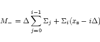
| M-' |
= |
 |
|
| |
|
.$](/articles/aa/full/2002/20/aa1942/img296.gif) |
(A.13) |
The mass fluxes can be written as:
 |
(A.14) |
where
 is an estimate of the linear density at the interface, the expression of which depends on the
numerical method (Stone & Norman 1992). To lowest order in
is an estimate of the linear density at the interface, the expression of which depends on the
numerical method (Stone & Norman 1992). To lowest order in
 ,
the mass variation can be expressed, after
a few transformations, and assuming F0=0, as:
,
the mass variation can be expressed, after
a few transformations, and assuming F0=0, as:
![\begin{figure}
\par\includegraphics[width=8.1cm,clip]{seperr.ps}
\end{figure}](/articles/aa/full/2002/20/aa1942/Timg303.gif) |
Figure A.3:
Relative error on the co-orbital corotation torque
in the shearing sheet, as a function of resolution (number of zones in
the horseshoe region half-width). The dotted and dashed lines are respectively
for the worst case and a conservative case for the runs presented here
(see text for details). |
This mass variation necessarily corresponds to the separatrix crossing mass, since F0=0.
One can get an estimate of this mass variation assuming
 (a reasonable assumption in the case of a radial
viscous drift) and writing
(a reasonable assumption in the case of a radial
viscous drift) and writing
 (in which case one
has to assume that
(in which case one
has to assume that
 ,
a reasonable assumption for the case of interest here).
One is then led to:
,
a reasonable assumption for the case of interest here).
One is then led to:
 |
(A.16) |
where
 is the x value of the zone center. One can therefore write:
 |
(A.17) |
from which one can infer:
 |
(A.18) |
where
 is the inner mass when the separatrix crosses the zone center. Equation (A.18) shows that the inner mass
at the top (
is the inner mass when the separatrix crosses the zone center. Equation (A.18) shows that the inner mass
at the top (
 )
and the bottom (
)
and the bottom (
 )
of the zone are the same, from which one
can conclude that, although some
mass can cross the separatrix as its sweeps the zone, there is no net effect as it sweeps the entire zone from one interface
to the other. As a consequence,
the maximum amount of mass that can cross the separatrix as it sweeps an arbitrary number of zones is
)
of the zone are the same, from which one
can conclude that, although some
mass can cross the separatrix as its sweeps the zone, there is no net effect as it sweeps the entire zone from one interface
to the other. As a consequence,
the maximum amount of mass that can cross the separatrix as it sweeps an arbitrary number of zones is
 .
Denoting with
.
Denoting with
 the error on the separatrix position, which is defined as:
 ,
one is led to
the following relation:
,
one is led to
the following relation:
 |
(A.19) |
The worst case is obtained for
 ,
i.e. when the separatrix lies on the edge of a fully emptied gap,
and when this edge is not resolved (i.e. when the density falls abruptly from
to 0 from one zone to its neighbor). It
should be stressed that this situation is far from being met in the simulations presented here. Even in this worst case, the
maximal error on the separatrix position will be:
,
i.e. when the separatrix lies on the edge of a fully emptied gap,
and when this edge is not resolved (i.e. when the density falls abruptly from
to 0 from one zone to its neighbor). It
should be stressed that this situation is far from being met in the simulations presented here. Even in this worst case, the
maximal error on the separatrix position will be:
 ,
whereas in a more reasonable case for which
,
whereas in a more reasonable case for which
 will typically amount to a small fraction of
  ,
the maximal error on the separatrix position will be a fraction of
,
the maximal error on the separatrix position will be a fraction of
 .
The worst case is displayed in Fig. A.3 with dotted lines, while the conservative case
where
.
The worst case is displayed in Fig. A.3 with dotted lines, while the conservative case
where
 ,
obtained for
,
obtained for
 and H=0.03 in the normal resolution runs, is displayed
with dashed lines. It is worth noting that the separatrix error is much smaller than this conservative estimate, in particular for
small planet masses, which hardly perturb the disk density profile, and for which
is the smallest. One can conclude
from Fig. A.3 that the corotation torque
is described with an accuracy better than 15% as soon as
and H=0.03 in the normal resolution runs, is displayed
with dashed lines. It is worth noting that the separatrix error is much smaller than this conservative estimate, in particular for
small planet masses, which hardly perturb the disk density profile, and for which
is the smallest. One can conclude
from Fig. A.3 that the corotation torque
is described with an accuracy better than 15% as soon as
 .
Although this condition is not met for the smallest mass planets in the normal resolution runs presented here, the corotation
torque, which on average for
.
Although this condition is not met for the smallest mass planets in the normal resolution runs presented here, the corotation
torque, which on average for
 numerical effects tend to overestimate, is never found to be large enough to
cancel out the differential Lindblad torque for these objects. Therefore, one can conclude that even with a relatively small
number of mesh rings involved in the co-orbital region, the code used here can describe with a reasonable precision the dynamics
of the co-orbital corotation torque, and that whenever the planet mass is too small for the dynamics of this region to be
correctly described (for the resolution and parameter set used here),
the corotation torque is too small to significantly affect the migration anyway (one recovers the linear regime, see Sect. 1 for details).
numerical effects tend to overestimate, is never found to be large enough to
cancel out the differential Lindblad torque for these objects. Therefore, one can conclude that even with a relatively small
number of mesh rings involved in the co-orbital region, the code used here can describe with a reasonable precision the dynamics
of the co-orbital corotation torque, and that whenever the planet mass is too small for the dynamics of this region to be
correctly described (for the resolution and parameter set used here),
the corotation torque is too small to significantly affect the migration anyway (one recovers the linear regime, see Sect. 1 for details).
Up: The co-orbital corotation torque
Copyright ESO 2002
![\begin{figure}
\par\includegraphics[width=8.7cm,clip]{resol1.eps}
\end{figure}](/articles/aa/full/2002/20/aa1942/img268.gif)

![$\displaystyle \times\left[\sum_{i=0}^{i_{\rm M}}i^3+(i_{\rm M}+1)^3\left(\frac{x_{\rm s}}{\Delta}-i_{\rm M}-\frac 12\right)\right]\cdot$](/articles/aa/full/2002/20/aa1942/img284.gif)
![\begin{figure}
\par\includegraphics[width=8.8cm,clip]{resol2.eps}
\end{figure}](/articles/aa/full/2002/20/aa1942/img289.gif)
![\begin{figure}
\par\includegraphics[width=8.1cm,clip]{seperr.ps}
\end{figure}](/articles/aa/full/2002/20/aa1942/img303.gif)