next previous
Up: Photometric redshifts from evolutionary


Subsections

3 Photometric redshifts with evolution

3.1 The HDF-N galaxy sample

The Hubble Deep Field North (HDF-N) catalog (Williams et al. 1996) was chosen to test the evolution factor. Spectroscopic redshifts were measured carefully by Cohen et al. (2000), with some additions and corrections in Cohen (2001). FSLY give photometric data for the HDF-N objects and Fernández-Soto et al. (2001a) give a correspondence between their objects and the objects in Cohen et al. (2000). We exclude from the sample galaxies with negative fluxes. The remaining selected sub-sample contains 136 galaxies with redshifts distributed from 0 to 5.6.

The HDF-N sample presents a series of advantages to explore the accuracy of our method and to compare it to others. With a large redshift range ( $0 \le z \le 5.6$), the sample data acquired with the WFPC2/HST camera is one of the deepest (down to B=29) with an extent over the wavelength range from about 3000 Å to 8000 Å  with the filters F300W, F450W, F606W, and F814W (hereafter called U, B, V, I). Moreover the near-infrared standard Johnson-Cousins J, H and $K_{\rm s}$ (hereafter K) colors listed in FSLY from Dickinson (1998) were observed at the KPNO/4 m telescope. The calibration used is AB magnitudes.
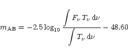
\begin{displaymath}m_{{\rm AB}}=-2.5\log_{10}\frac{\displaystyle{\int F_{\nu}
\,...
...u}\,{\rm d}\nu}}{\displaystyle{\int T_{\nu}\,{\rm d}\nu}}-48.60\end{displaymath}

with $F_{\nu}$ in ergs-1cm$^{-2}\,$Hz-1. $T_{\nu}$ is the transmission of the filter.

A further advantage is the benefit of spectroscopic redshifts of the selected sub-sample, as given by Cohen (2001). This allows a statistical comparison with our photometric redshifts and an estimation of the dispersion. Another advantage of this sample is the possibility of measuring the type-dependent evolution factor by comparing our results with the FSLY's results, since the latter authors propose photometric redshift determinations based on a maximum likelihood analysis and 4 spectral types without any evolution effect.

3.2 The spectroscopic-z-photometric-z plane

Figure 2 presents the plane $z_{{\rm spe}}$- $z_{\rm phot}$  resulting from our fit of the HDF-N sample with PÉGASE templates.
  \begin{figure}
\par\includegraphics[width=8.3cm,clip]{MS2109f3.eps}\end{figure} Figure 2: Comparison of photometric redshifts (points with error bars) predicted by the model Z-PEG.1 to spectroscopic redshifts of the selected HDF-N sample. The solid line of slope = 1 shows the case of equality for comparison. The dotted line is the linear regression of our photometric redshifts if we exclude the points with $\vert z_{{\rm Z-PEG}}-z_{{\rm spe}}\vert \geq 1$. Predictions are computed with IGM absorption from Madau et al. (1996) and ISM reddening according to PÉGASE algorithms. When two solutions or more are found (degeneracy), the error bars are linked by a dotted line. The squares are objects with discordant redshifts also pointed out by Fernández-Soto et al. (2001a).

3.3 Evolution factors

3.3.1 Average evolution factor on ${\vec{z}_{{phot}}}$

We compare our best results $z_{{\rm Z-PEG}}$, from the evolutionary model Z-PEG.1 (selected from the variety of models in Table 2) to photometric redshifts $z_{{\rm FS}}$estimated by FSLY. These authors only took into account k-corrections of the galaxy spectral distributions from Coleman et al. (1980) while we simultaneously compute the k- and e- correction factors at any z. Figure 3 shows the difference for each galaxy of the sample. Lines trace the median values of the difference of $z_{{\rm FS}}$ with Z-PEG.1, and $z_{{\rm spe}}$  values respectively. The zero value (difference to $z_{{\rm FS}}$) is plotted for comparison. A systematic effect is observed for $z \geq 1.5$. The evolution effect is measured around $<z_{{\rm Z-PEG}}-z_{{\rm FS}}>$ = 0.2, independent of type. The median[*] value $<z_{{\rm Z-PEG}}-z_{{\rm spe}}>$ = - 0. 03is measured and remains inside the error bars. Evolution effects are more important for distant galaxies and an appropriate evolutionary code is required for such estimates.
  \begin{figure}
\par\includegraphics[clip,width=8.3cm,clip]{MS2109f4.eps}\end{figure} Figure 3: Crosses are differences $z_{{\rm Z-PEG}}-z_{{\rm FS}}$. For $z_{{\rm spe}}> 1.5$, the evolution factor is measured by the distance between the dotted and full lines, respectively the median value $<z_{{\rm Z-PEG}}-z_{{\rm FS}}>$and 0. $z_{{\rm FS}}$ are the FSLY's determinations. The dashed line is the median value $<z_{{\rm spe}}-z_{{\rm FS}}>$. For $z_{{\rm spe}}<1.5$, the evolution factor has the same magnitude as the error bars.

3.3.2 Determination of galaxy spectral types

Our best fit gives a minimal $\chi ^2$ for a triplet (age, redshift, type), so that we can deduce the spectral type of the observed galaxies by comparing to the SEDs of 9 different types. The comparison of types derived by Z-PEG.1 and by FSLY is shown in Fig. 4. In most cases, "earlier type'' galaxies are found with Z-PEG.1, particularly at high redshifts. This effect is expected from evolution scenarios because, when considering only the k-correction, FSLY would find an evolved spiral galaxy when Z-PEG.1 finds a young elliptical galaxy. A better definition of the morphological properties of galaxies in the near future will help us to arrive at a conclusion.


  \begin{figure}
\par\includegraphics[width=8.3cm,clip]{MS2109f5.eps}\end{figure} Figure 4: Comparison of our spectral type estimates to FSLY's. The values are $type_{\textrm{\it \tiny Z-PEG}}-type_{\textrm{\tiny FS}}$ assuming the following values for the spectral types (type 0: starburst, 1: elliptical, 2: S0, 3: Sa, 4: Sb, 5: Sbc, 6: Sc, 7: Sd, 8: Im).


Table 2: The variety of Z-PEG models is tabulated with the adopted constraints (IGM absorption, near-infrared JHK filters and age). Statistical results (mean difference and dispersion) are given in last columns. A comparison to FSLY and Massarotti et al. (2001b) results is also given. The $\overline {\Delta z}$ and $\sigma $ are computed using primary and secondary solutions for Z-PEG models (see  Sect. 2.2), and primary solutions only for FSLY and MIBV models.
Z-PEG Model IGM abs. UBVI JHK age constraint   z<1.5 all z Fig.
1 x x x x $\overline {\Delta z}$$\,=\,$-0.0214 -0.0844 2
          $\sigma_z$$\,=\,$ ${\bf0.0980}$ ${\bf0.4055} $  
2 x x x   $\overline {\Delta z}$$\,=\,$0.0251 -0.0621 5
          $\sigma_z$$\,=\,$ ${\bf0.1156}$ ${\bf0.4441} $  
3   x x   $\overline {\Delta z}$$\,=\,$0.0252 -0.0589 5
          $\sigma_z$$\,=\,$0.1156 0.5738  
4 x x     $\overline {\Delta z}$$\,=\,$0.1273 -0.0040 7
          $\sigma_z$$\,=\,$0.3179 0.5840  
FSLYa x x x   $\overline {\Delta z}$$\,=\,$-0.0037 -0.0579  
          $\sigma_z$$\,=\,$0.1125 0.2476  
MIBVb x x x   $\overline {\Delta z}$$\,=\,$0.026    
          $\sigma_z$$\,=\,$0.074    
a Results with FSLY's $z_{\rm phot}$ on the same sample, for comparison, using only primary solutions.
b Results from Massarotti et al. (2001b) with PÉGASE and additional starburst component on a similar sample,
for comparison, using only primary solutions.


next previous
Up: Photometric redshifts from evolutionary

Copyright ESO 2002