The weak distortion of background sources produced by gravitational lenses can be used to construct the projected mass distribution of the lens (see Tyson et al. 1990; Mellier 1999; Bartelmann & Schneider 2000). The excellent quality of the FORS1 data-set, especially the depth and the seeing, enabled us to accurately correct for many of the non-gravitational distortions of the image (PSF shear/smear) and also explore in some detail issues like fidelity of reconstructed mass features. To do this two teams, using different source selection criteria and different mass reconstruction schemes, independently produced maps of the mass distribution in MS 1008-1224.
Method 1
The IMCAT weak-lensing analysis package has been made publicly available at the URL http://www.ifa.hawaii.edu/~kaiser by Kaiser and his collaborators (Kaiser et al. 1995; Luppino & Kaiser 1997). The specific version used was the one modified and kindly made available to us by Hoekstra (see Hoekstra et al. 1998). A description of the analysis including measurement of the galaxy polarization, correction for smearing by and anisotropy of the PSF and the shear polarizability of galaxies and the expression for the final shear estimate have already been given by Hoekstra et al. (1998) and references therein and will not be repeated here.
The PSF anisotropy varied across the image and was about 0.015 (shape polarisation). The variation across the image was determined and corrected (separately in each band) using 50-60 stars scattered all over the CCD. The correction resulted in a mean residual polarisation of 0.0002 (rms = 0.004) for these PSF stars.
The maximum probability algorithm of Squires & Kaiser (1996), with K = 20(number of wave modes) and
![]() (the regularisation parameter), was
used to reconstruct the mass distribution from the shear field. Our analysis
differs from that of Hoekstra et al. only in the weighting of the data at the
final stage (described next).
(the regularisation parameter), was
used to reconstruct the mass distribution from the shear field. Our analysis
differs from that of Hoekstra et al. only in the weighting of the data at the
final stage (described next).
While this method works quite well it has the disadvantage that the error weighting and the Gaussian smoothing are coupled to each other. Decreasing the Gaussian smoothing scale (to investigate finer structure in the mass map) reduces the effectiveness of the all important error weighting; in the limiting case when the Gaussian smoothing scale includes just one background source (on the average) there is no error weighting at all. Since lensing inversion is a highly non-linear process and the individual shear values were dominated by the errors on them, this resulted in the final reconstructed mass distributions being considerably dependent on the smoothing scale used. Often we could not discern any signal at all in the mass map when small smoothing scales were used.
To remedy this, apart from
![]() we also calculated the error
on it,
we also calculated the error
on it,
![]() /[
/[
![]() ]2 and used this to weight the shear
values in the mass reconstruction algorithm. This removed the dependence of
error weighting on the smoothing scale and made it possible to make mass maps
with very small smoothing scales to (i) confirm that
the lower resolution mass maps could be obtained by a post-reconstruction
smoothing of the higher resolution map which indicated that our error-weighting
and hence error estimates were correct, (ii) check the stability of the
individual features seen in the mass reconstruction and (ii) investigate the
mass distribution in better detail.
]2 and used this to weight the shear
values in the mass reconstruction algorithm. This removed the dependence of
error weighting on the smoothing scale and made it possible to make mass maps
with very small smoothing scales to (i) confirm that
the lower resolution mass maps could be obtained by a post-reconstruction
smoothing of the higher resolution map which indicated that our error-weighting
and hence error estimates were correct, (ii) check the stability of the
individual features seen in the mass reconstruction and (ii) investigate the
mass distribution in better detail.
However, it has disadvantages as well. Any hole in the shear field (caused
by a bright star, for example) is filled in with zeros by the algorithm
leading to strong ripples and negative peaks in the reconstucted image.
As a result one sometimes finds egregious artifacts which are 5-10 times
larger than the noise. In general, the noise calculated over small regions
(i.e. the "true" noise which avoids large scale correlated fluctuations) is
3-5 times smaller than an rms calculated over a large area including ripples
and all. However, this latter quantity is perhaps more appropriate for
determining the
significance of the features in the mass maps and is the value listed in the
figure captions. It must be noted that this is not the rms of a Gaussian
random distribution and hence the usual rules of thumb and relationships of
Gaussian distributions (e.g. >![]() is significant) may not always be
appropriate. We discuss below some of the ways, some heuristic and others more
solid, in which we can deduce the reliability of the features seen in the mass
reconstruction:
is significant) may not always be
appropriate. We discuss below some of the ways, some heuristic and others more
solid, in which we can deduce the reliability of the features seen in the mass
reconstruction:
(i) The Curl-map: the shear field is a function of the gradient of the
gravitational potential and so a mass map made from the curl of the shear
field (effectively replacing ![]() by
by ![]() and
and ![]() by
by
![]() )
must produce a structure-less noise map (Kaiser 1995) in the
absence of systematic errors in the shear field. Thus, such a Curl-map may be
expected to indicate the location and intensity of artifacts. Further, since
the Curl-map is essentially free of source regions most of its pixels can be
used to get a good estimate of the "large-scale'' rms discussed earlier.
)
must produce a structure-less noise map (Kaiser 1995) in the
absence of systematic errors in the shear field. Thus, such a Curl-map may be
expected to indicate the location and intensity of artifacts. Further, since
the Curl-map is essentially free of source regions most of its pixels can be
used to get a good estimate of the "large-scale'' rms discussed earlier.
(ii) Bootstrap techniques.
(iii) Compare mass maps made with different smoothing scales: features which
vary from one scale to another in an inconsistent manner are likely to be
artifacts.
(iv) Compare mass maps made with data from different bands: the shape of each
lensed galaxy is approximately (but not exactly) the same in every band though
the final shape should be different due to different PSFs and photon noise,
especially for faint sources. It is necessary that a feature, in
order to be considered real, should be of similar shape and intensity (within
errors) in all the bands. Since the noise is so much stronger than the shear
signal reproducing the same features in all the bands is an indication that
PSF corrections and noise weighting were handled appropriately. Of course, this
check is not sufficient to prove that the features are real since intrinsic
ellipticities and locations of the background galaxies are similar/same in
all the bands (see next point).
(v) Random shuffling of the Shear: the shear is sampled only at the positions
of the background sources. Therefore, this multiplicative sampling function
leaves its own convolved footprint on the mass map. However one can get a
qualitative idea of the effect by keeping the positions fixed and randomly
shuffling the observed shear values among them. Obviously this should again
result in a structure-less noise map if there were no systematics introduced
by the sampling function and the FFT.
(vi) An inspection of the location and significance (in terms of rms) of the
negative peaks on the mass map itself.
Method 2
This method also used the raw IMCAT software from Kaiser's home page (see
previous method) with some minor modifications for estimating the shear field.
The mass reconstruction was done using the maximum likelihood estimator
developed by Bartelmann et al. (1996) with the finite difference scheme
described in Appendix B of Van Waerbeke et al. (1999). The
reconstruction was not regularised and hence the resulting mass maps were
noisier than those obtained from Method 1. However, as pointed out Van Waerbeke
et al. (1999) and Van Waerbeke (2000) the advantage of method 2 is that the noise
can be described analytically in the weak lensing approximation. When galaxy
ellipticities are smoothed with a Gaussian window
 |
(1) |
 |
(2) |
The mass reconstructions from B, V, R and I data using the first method are
shown in Fig. 7 (30 arcsec smoothing scale) and Fig. 8 (15 arcsec smoothing scale).
![\begin{figure}
\par\includegraphics[width=10cm,clip]{ms1776f7.eps}
\end{figure}](/articles/aa/full/2002/12/aa1776/img98.gif) |
Figure 7:
Mass reconstruction of MS 1008-1224 from B, V, R and
I images using the algorithm of Squires & Kaiser (1996) - Method 1 in the text
- and a Gaussian smoothing of 30 arcsec. The iso-convergence contour
interval is
|
![\begin{figure}
\par\includegraphics[width=9cm,clip]{ms1776f8.eps}
\end{figure}](/articles/aa/full/2002/12/aa1776/img99.gif) |
Figure 8:
Mass reconstruction of MS 1008-1224 from B, V, R and
I images using the algorithm of Squires & Kaiser (1996) - Method 1 in the
text - and a Gaussian smoothing of 15 arcsec. The bottom-left plot is the
average of the 4 upper plots while the bottom-right is the average of the
Curl-map in each band. The iso-convergence contour interval is |
The lower resolution reconstructions (Fig. 7) are very similar in
shape as well as magnitude of the peak (![]() 5 per cent variation). The
main features are a central mass condensation which seems to be
elongated in the north-south direction, a fainter extension towards the north
and a ridge leading off towards the north-east from the main component. The
prominent cross at (222, 222) marks the location of the cD galaxy.
5 per cent variation). The
main features are a central mass condensation which seems to be
elongated in the north-south direction, a fainter extension towards the north
and a ridge leading off towards the north-east from the main component. The
prominent cross at (222, 222) marks the location of the cD galaxy.
The higher resolution image (Fig. 8) clearly resolves the principal mass component into 2 peaks separated along (mostly) the north-south direction. Once again, it may be noted that the structures are similar in all the bands. We also note that the northern peak appears to be marginally higher than the southern one in all images. This montage (Fig. 8) also includes an average of the mass maps in the 4 bands (bottom-left). The concentric circles denote the annuli within which the mass was estimated to determine the radial profile. They are centred on the centroid of the mass distribution (the black dot) determined from the average of the lower resolution maps (Fig. 7). It must be noted that averaging the mass distribution from all the 4 bands does reduce the amplitude of spurious ripples relative to the more stable mass peaks but not by a factor of 2; for one, the noise is not Gaussian and for another, averaging the shear field with data from different bands reduces the photon noise but not the noise due to intrinsic galaxy ellipticity.
Also shown on the same plot is an average of the Curl-maps made in each of the 4 bands (bottom-right). There were two very bright stars in the MS 1008-1224 field which were masked on the FORS1 images. The thick curved lines delineate the extent of these masks from where no shear data was available. These holes in the shear field led to strong spurious peaks and ripples in the mass map.
The two mass components at the centre are the most significant features in all the maps. Their stability across the different bands and smoothing scales as well as their high level of significance is a strong indicator that they are real features.
An inspection of the mass maps in Figs. 7 and 8 clearly shows that the strongest negative peak in each is in the region of the masks. Further, the north-eastern ridge mentioned earlier is along the boundary of one of the masks, its intensity varies from band to band (in contrast to the 2 principal mass components) and is very prominent in the Curl-map. So we concluded that it was a spurious feature spawned by the FFT and the masks. It was heartening to note that the strong spurious peaks generated by the masks were confined to their immediate vicinity and that much of the Curl-map, especially the lower half, mimics random noise with no strong features.
It is more difficult to determine if the faint but extensive signal leading to the north has a basis in reality. Given its faintness its considerable fluctuation from one map to another is only to be expected. But to a greater or lesser extent it is present in every single plot including others (not shown in this paper) obtained from different combinations of smoothing scale and wave-modes. So, we tentatively suggest that it is real but we shall not attempt to mine it for any further information. We only note that the cluster number and luminosity density distributions (Fig. 6) also show secondary peaks towards the north.
Another point that we shall discuss in more detail a little later is the offset between the cD galaxy and the centroid of the mass distribution.
The mass reconstructions obtained using method 2 are shown in Figs. 9 and 10 (20 and 15 arcsec smoothing scales,
respectively).
![\begin{figure}
\par\includegraphics[width=6.8cm,clip]{ms1776f10.eps}
\end{figure}](/articles/aa/full/2002/12/aa1776/img103.gif) |
Figure 10:
High resolution mass reconstruction of MS 1008-1224
using Method 2 and a smoothing scale of 15 arcsec. The final plot was
obtained by averaging the mass reconstructions in the 4 different bands. This
averaging reduces the noise due to measurement error by a factor of 2 (but not
that due to intrinsic ellipticity). The iso-convergence ( |
We compared the two methods quantitatively by carrying out a Pearson's r-test
(Press et al. 1992) on the high resolution mass reconstructions (the Fig. 8 "Mass-av'' image of method 1 and Fig. 10
"I+R+B+V'' image of method 2). We obtained an r-coefficient of 0.837 for
on-signal pixels and r = 0.298 for off-signal pixels. The smallest
rectangle enclosing the 3![]()
![]() contours of both images defined
the on-signal region while the bottom quarter of the image was used for the
off-signal region since this was the only clean area lacking the spurious
features generated by the large masks in the upper half of the images (see
Fig. 8 bottom-right plot). The on-signal correlation is
very high and as expected much higher than the off-signal correlation.
However the off-signal is still correlated because many galaxies are
common in both methods (locations and shapes are the same), which will
lead to correlated structures at the noise level throughout the map.
Joffre et al. (2000) also measured a similar high correlation in the case of
Abell 3667 even after masking the statistically significant regions of the
mass distribution.
contours of both images defined
the on-signal region while the bottom quarter of the image was used for the
off-signal region since this was the only clean area lacking the spurious
features generated by the large masks in the upper half of the images (see
Fig. 8 bottom-right plot). The on-signal correlation is
very high and as expected much higher than the off-signal correlation.
However the off-signal is still correlated because many galaxies are
common in both methods (locations and shapes are the same), which will
lead to correlated structures at the noise level throughout the map.
Joffre et al. (2000) also measured a similar high correlation in the case of
Abell 3667 even after masking the statistically significant regions of the
mass distribution.
We used Method 2 to quantify the magnitude and significance of this
offset. The best way for measuring the significance of the offset would have
been to use an independent parametric model for the mass distribution and a
parametric bootstrap method to generate a large number of mass reconstructions
with different noise realisations and then measure the dispersion of the cD-mass centroid offset. Since such a model was not available we used the
reconstructed mass map itself as the model.
Combining different realisations of the noise (using the noise model of Eq. (2)),
galaxy positions and intrinsic ellipticities we generated 5000 simulated
datasets based on the I-band data at three different smoothing scales of 20, 30
and 40 arcsec. Figure 11 illustrates the positional
stability one may expect in mass reconstructions and the numbers in Table 2 quantify the statistical significance of the offset.
|
|
|
|
|
|
|
|
| Prob(
|
0.46 | 0.79 | 0.44 | 0.86 | 0.64 | 0.92 |
| Prob(
|
0.21 | 0.48 | 0.20 | 0.68 | 0.30 | 0.73 |
Clearly, mass features move around on scales of ![]() 10 arcsec and this
effect, naturally, increases with decrease of smoothing scale. One of the
lessons we draw from this analysis is that squeezing finer mass details from
the shear data is possible but at the expense of considerable flakiness in the
positions of the features. It is important to reconstruct mass maps
using various smoothing scales before attempting an interpretation of the same.
Finally, the cD galaxy is offset to the south of the mass centroid by
19+22.5-18.5 arcsec (confidence level, CL = 90%); or, the cD
is at least 5 arcsec (CL = 90%) south of the mass centroid.
10 arcsec and this
effect, naturally, increases with decrease of smoothing scale. One of the
lessons we draw from this analysis is that squeezing finer mass details from
the shear data is possible but at the expense of considerable flakiness in the
positions of the features. It is important to reconstruct mass maps
using various smoothing scales before attempting an interpretation of the same.
Finally, the cD galaxy is offset to the south of the mass centroid by
19+22.5-18.5 arcsec (confidence level, CL = 90%); or, the cD
is at least 5 arcsec (CL = 90%) south of the mass centroid.
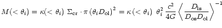
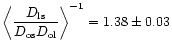
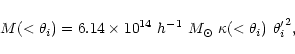
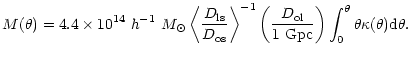
The mass from weak shear,
![]() ,
may be obtained from Aperture Mass
Densitometry or the
,
may be obtained from Aperture Mass
Densitometry or the ![]() -statistics described by Fahlman et al. (1994) and
Squires & Kaiser (1996). In brief, the average tangential shear in an annulus
is a measure of the average density contrast between the annulus and the region
interior to it; i.e. the average convergence
-statistics described by Fahlman et al. (1994) and
Squires & Kaiser (1996). In brief, the average tangential shear in an annulus
is a measure of the average density contrast between the annulus and the region
interior to it; i.e. the average convergence ![]() (
(![]()
![]() ), the ratio of the surface mass density to the critical surface
mass density for lensing, as a function of the radial distance
), the ratio of the surface mass density to the critical surface
mass density for lensing, as a function of the radial distance ![]() is given
by
is given
by
 |
(3) |
From Eq. (3), one can derive the average convergence within a series of apertures
of radii ![]() ,
,
![]()
 |
(4) |
 |
(5) |
 Gpc
(
Gpc
( |
(6) |
The radial profile of the shear is shown in Fig. 12.
![\begin{figure}
\par\includegraphics[width=7.9cm,clip]{ms1776f12.eps}
\end{figure}](/articles/aa/full/2002/12/aa1776/img133.gif) |
Figure 12:
Radial profile of shear in the MS 1008-1224 field.
The filled circles are the tangential shear in successive annuli centered on the
mass centroid (see Fig. 8). The open circles represent the Curlof the shear field which are expected to be (and are) distributed around zero
if the shear field was due to gravitational lensing.
The bars respresent
|
The mass profile inferred from the shear is shown in Fig. 13 as
a series of filled circles along with the error bars.
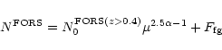
The combined effect of deflection and magnification of light, results in a
modification of the number density of galaxies seen through the lensing cluster.
In the case of a circular lens, the galaxy count at a radius ![]() is
is
 |
(7) |
We considered as foreground those galaxies at
![]() and as
background (lensed) those at
and as
background (lensed) those at
![]() (see Sect. 3.2). We
minimized misclassification by considering only those which had a good
photometric redshift solution (hyperz fit
(see Sect. 3.2). We
minimized misclassification by considering only those which had a good
photometric redshift solution (hyperz fit
![]() ). To be consistent with
the shear analysis, we considered only the
). To be consistent with
the shear analysis, we considered only the
![]() (method 1) and
(method 1) and
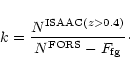
![]() (method 2) samples. The galaxy counts slopes for the 2 samples were found to be 0.192 and 0.233, respectively, suggesting that
depletion would be significant in the FORS1 and ISAAC data.
(method 2) samples. The galaxy counts slopes for the 2 samples were found to be 0.192 and 0.233, respectively, suggesting that
depletion would be significant in the FORS1 and ISAAC data.
Figure 14 shows the projected number density of galaxies having
good photometric redshifts from BVRIJK data and in the magnitude range
![]() .
.
The modification of the radial distribution of galaxy counts (i.e., the
magnification bias) probes the amplitude of the projected mass density. In the
weak lensing regime the relation simplifies to:
| = | (8) | ||
| (9) |
 |
(10) |
(i) The depletion extends beyond the ISAAC field.
(ii) A lensed background cluster:
we detected a significant enhancement of galaxy number density on the
bottom-right (hereafter Q4) quadrant of the ISAAC field (Fig. 14, lower panel). A visual inspection of the FORS1 images showed
faint and distorted galaxies between a radius of 50 and 80 arcsec from the
centre of depletion. We compared the photometric redshift distribution of
galaxies in Q4 with that from the other three quadrants (Q1-3). The
difference between the (area-normalised) galaxy numbers in Q4 and Q1-3
are plotted in Fig. 15.
So we tried to determine the asymptotic zero-point for ISAAC by extrapolating
from the FORS1 field as a whole. We selected galaxies from the FORS1 field
which were fainter than the brightest cluster members and outside the cluster
sequence on the Colour-Magnitude plot. We then computed the radial galaxy number
density from the FORS1 data within the ISAAC area, excluding the the background
cluster. Figure 16 shows the depletion curves for the FORS1
field as well as for the ISAAC subsamples with photometric redshifts.
 |
(11) |
For the
![]() sample in the ISAAC field we have
sample in the ISAAC field we have
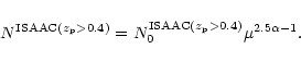 |
(12) |
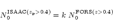 |
(13) |
 |
(14) |
In conclusion, despite the very good data set this method is still saddled with large errors. Depletion analysis is in principle very simple (just counting galaxies) and a neat way of avoiding the mass sheet degeneracy of shear analysis but is plagued by cosmic variance, background clustering and, as we have demonstrated here, the necessity of having complete redshift samples.
Copyright ESO 2002
![\begin{figure}
\par\includegraphics[width=6.1cm,clip]{ms1776f9.eps}
\end{figure}](/articles/aa/full/2002/12/aa1776/img102.gif)
![\begin{figure}
\par\includegraphics[width=7cm,clip]{ms1776f11.eps}
\end{figure}](/articles/aa/full/2002/12/aa1776/img105.gif)
![\begin{figure}
\par\includegraphics[width=5.9cm,clip]{ms1776f13.eps}
\end{figure}](/articles/aa/full/2002/12/aa1776/img136.gif)
![\begin{figure}
\par\includegraphics[width=6.6cm,clip]{ms1776f14.eps}
\end{figure}](/articles/aa/full/2002/12/aa1776/img140.gif)
![\begin{figure}
\par\includegraphics[width=6.8cm,clip]{ms1776f15.eps}
\end{figure}](/articles/aa/full/2002/12/aa1776/img148.gif)
![\begin{figure}
\par\includegraphics[width=5.75cm,clip]{ms1776f16.eps}
\end{figure}](/articles/aa/full/2002/12/aa1776/img151.gif)