3 Results

3.1 Newly discovered objects

The central part of CB34 in the continuum subtracted (1, 0) S(1) line of molecular hydrogen is shown in Fig. 1. The lowest H₂ contours are two standard deviations above the noise in the sky level. The marked objects are taken from Huard et al. (2000; crosses "+''), Moreira & Yun (1995; "$\times$''s), Yun et al. (1996; "diamonds'') and Yun & Clemens (1994; "triangles'') which are overlaid using the SIMBAD online data base.

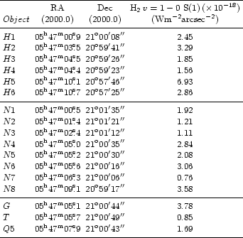
Newly found H₂ objects are marked with the letters H1-H6, N1-N6, G, T and Q5. The objects Q1-Q4 are H₂ emission objects discovered by Moreira & Yun (1995). Our knot Q5 appears to be associated with Q1-Q4.

An estimate of the surface brightness averaged over a 2 $\hbox {$^{\prime \prime }$ }$ aperture of the newly discovered emission objects is given in Col. 4 of Table 1. Columns 2 and 3 of Table 1 contain the right ascension and declination of the objects.

  

Table 1: New object positions and fluxes.

3.2 Infrared photometry

The sky conditions during the observations were less than optimal and non-photometric in particular, which does not allow us to derive independent absolute photometry. Here, we estimate fluxes of the emission objects in CB34 from a relative photometry obtained from a comparison with the same knots which were found by Alves & Yun (1995).

For the $JHK_{\rm s}$ photometry, we use the IRAF DAOPHOT routine (Stetson 1987) to identify stars which are simultaneously present in the J, H, and $K_{\rm s}$ frames and to obtain instrumental stellar magnitudes. Then, instrumental magnitudes were compared with the same objects' absolute magnitudes obtained from the work of Alves & Yun (1995) in order to detect magnitude transformation constants. Then, using the same constants for all our detected stars, the instrumental magnitudes were transformed to absolute magnitudes. This transformation method yields errors of no more than 15% in comparison with the results from Alves & Yun (1995), although in some cases the values are identical (cf. objects A, C and D).

Figure 2 identifies the 14 most reddened objects found in this way, labelled with the same letters A-S as used by Alves & Yun (1995). These objects are represented by filled circles in the (J-H) and (H-K) colour-colour diagrams of Fig. 3. The solid line in the figure represents the location of the un-reddened main-sequence stars (Koornneef 1983). The two parallel dashed lines are the reddening vectors which define the reddening band for normal stellar photospheres. Objects with colours that fall outside and to the right of this band are sources with intrinsic infrared excess emission (Lada & Adams 1992).

Figure 2: Isophotes of the central region of CB34 in $K_{\rm s}$ covering an area of about 2.5 $\times$ 2.5 arcmin2. East is left, north is up. Letters A,B,C,D,E,F,G,K,L,M,N,P,Q and S are the 14 reddest objects. Notice Object S which has large [H-K] and is located at the edge of the cloud, suggesting that it is a background star.

Figure 3: Near-infrared colour-colour diagram for all sources detected in the J, H and $K_{\rm s}$ bands simultaneously. The solid line is the location of the un-reddened main-sequence stars (Koornneef 1983). Dashed lines are two parallels to the reddening vector which define the reddening band for normal stellar photospheres. Objects with (H-K) > 1.0 are marked with filled circles (see Figs. 2, 4 and 5). Crosses are objects with (H-K) $\le$ 1.0. Letters represent the same objects as in Fig. 2. The size of the error bars is shown in the lower right-hand corner.

Figure 4: Plot of the [H-K] colour as a function of projected angular distance to an estimated centre point object-E, which was chosen by visual examination of the cloud (cf. Figs. 1 and 2). The symbols are the same as described in Fig. 3.

Figure 5: Spatial distribution of all the sources seen in the 3 bands simultaneously. The offset centre is the object E.

Figure 4 shows the spatial distribution of all sources detected simultaneously in the J,H and $K_{\rm s}$ images. Those with (H-K) > 1.0 are represented by filled circles in Figs. 2, 4 and 5. Crosses mark objects with (H-K) $\le$ 1.0. From Figs. 4 and 5 one can derive a core radius of the Bok globule of approximately 50 $^{\prime \prime }$-60 $^{\prime \prime }$ which contains all those objects with (H-K) > 1.6.

A number of objects with large (H-K) are located at the edge of the cloud (cf. Fig. 3 in comparison with Figs. 2, 4 and 5). Those objects (cf. S, N and K) are probably background stars. Because of the large distance of 1500pc to the globule (Carpenter et al. 1995), 1-2 of the red stars located within the globule may be red foreground objects and not embedded. Objects C and G are located in the region of the [(J-H) vs. (H-K)]-plane which has been explained by disk emission (Strom et al. 1989) and are class II objects (Adams et al. 1987). Objects A, B, D, E, and L have large (H-K) and are located in the region of the diagram characterized by large extinction corresponding mostly to class I sources (Lada & Adams 1992).

The near-infrared colours of the objects A, B, C, D, E, G and L give us confidence that they are young stellar objects (YSOs), surrounded by varying amounts of circumstellar material, and that they formed recently as a part of ongoing star formation in the CB34 Bok globule. This is in good agreement with results from Alves & Yun (1995).