Figures 3 and 4 present the 12, 25, 60, and ![]() m background-subtracted IRAS co-added images of GF 17 and GF 20. The
m background-subtracted IRAS co-added images of GF 17 and GF 20. The ![]() m and
m and ![]() m images reveal few point sources toward GF 17 and GF 20. Some of these sources are confirmed young stellar objects (mostly T Tauri stars) associated with their parent cloud, while other sources are simply unrelated background and/or foreground objects. The locations of confirmed young stellar objects within each cloud are indicated by the filled star symbols. Of the eight T Tauri stars known to be associated with GF 17 (Schwartz 1977), only four are seen in our IRAS field. These are found in regions of visual extinction smaller than 1 mag (Andreazza & Vilas-Boas 1996), and distributed around the main core region of GF 17. Four of the five T Tauri stars associated with GF 20 are seen in our IRAS field. The strongest
m images reveal few point sources toward GF 17 and GF 20. Some of these sources are confirmed young stellar objects (mostly T Tauri stars) associated with their parent cloud, while other sources are simply unrelated background and/or foreground objects. The locations of confirmed young stellar objects within each cloud are indicated by the filled star symbols. Of the eight T Tauri stars known to be associated with GF 17 (Schwartz 1977), only four are seen in our IRAS field. These are found in regions of visual extinction smaller than 1 mag (Andreazza & Vilas-Boas 1996), and distributed around the main core region of GF 17. Four of the five T Tauri stars associated with GF 20 are seen in our IRAS field. The strongest ![]() m source, and almost coincident with the peak of
m source, and almost coincident with the peak of ![]() m emission, is the extremely active T Tauri star RU Lupi (Schwartz 1977). Andreazza & Vilas-Boas (1996) estimate the visual extinction to this source to be
m emission, is the extremely active T Tauri star RU Lupi (Schwartz 1977). Andreazza & Vilas-Boas (1996) estimate the visual extinction to this source to be
![]() mag from optical star counts. The remaining T Tauri stars are found in regions of visual extinction smaller than 1 mag (Andreazza & Vilas-Boas 1996).
mag from optical star counts. The remaining T Tauri stars are found in regions of visual extinction smaller than 1 mag (Andreazza & Vilas-Boas 1996).
The IRAS wide-field, high dynamic range images clearly reveal the filamentary nature of GF 17 and GF 20. The spatial distribution of dust emission in these globular filaments is not irregular in shape, but rather is extremely elongated. The ![]() m emission from GF 17 peaks at a main core region, and defines a filamentary region toward the east. In GF 20, the
m emission from GF 17 peaks at a main core region, and defines a filamentary region toward the east. In GF 20, the ![]() m emision peaks at a main core region associated with RU Lupi. A second strong peak of
m emision peaks at a main core region associated with RU Lupi. A second strong peak of ![]() m emission is located about
m emission is located about
![]() to the south of RU Lupi. A third peak of
to the south of RU Lupi. A third peak of ![]() m emission appears within the filamentary part of GF 20. Like GF 17, the filamentary structure in GF 20 is well delineated at
m emission appears within the filamentary part of GF 20. Like GF 17, the filamentary structure in GF 20 is well delineated at ![]() m, extending to the northeast, away from RU Lupi. Table 1 summarizes the
m, extending to the northeast, away from RU Lupi. Table 1 summarizes the ![]() m and
m and ![]() m peak fluxes of dust emission from selected regions within each cloud. The positions in Cols. 3 and 4 were derived from the
m peak fluxes of dust emission from selected regions within each cloud. The positions in Cols. 3 and 4 were derived from the ![]() m images. Columns 7, 8, and 9 give average dust temperatures, optical depths, and visual extinctions observed within each region.
m images. Columns 7, 8, and 9 give average dust temperatures, optical depths, and visual extinctions observed within each region.
| Peak Brightness | ||||||||
| (MJy ster-1) | ||||||||
| RA | Dec | T60/100 |
|
AV | ||||
| Cloud | Region | (1950) | (1950) | (K) | (
|
(mag) | ||
| (1) | (2) | (3) | (4) | (5) | (6) | (7) | (8) | (9) |
| GF 17 | main core |
|
|
4.8 | 15.4 | 43 | 0.7 | 0.4 |
| filament | 16 00 30 |
|
3.2 | 11.0 | 42 | 0.4 | 0.2 | |
| GF 20 | main core(a) | 15 53 30 |
|
3.4 | 17.1 | 31 | 3.1 | 0.7 |
| main core(b) | 15 53 40 |
|
4.4 | 17.2 | 30 | 2.8 | 0.6 | |
| filament | 15 55 00 |
|
2.3 | 12.1 | 33 | 1.6 | 0.4 | |
| filament | 15 56 00 |
|
1.8 | 10.0 | 32 | 1.5 | 0.4 | |
(a) South of RU Lupi.
(b) Associated with RU Lupi.
GF 17 and GF 20 share an interesting characteristic in their dust emission. Note that we do not see the clouds boundaries at 12 or ![]() m. This is unlike the
m. This is unlike the ![]() Ophiuchi cloud which has IR boundaries clearly delineated at both
Ophiuchi cloud which has IR boundaries clearly delineated at both ![]() m (
m (
![]() K) and
K) and ![]() m (
m (
![]() K), as shown by Jarrett et al. (1989). These authors concluded that the IR emission from
K), as shown by Jarrett et al. (1989). These authors concluded that the IR emission from ![]() Ophiuchi needs to be modeled as arising from two physically distinct populations of dust grains. Our IRAS images thus suggest that the IR emission from GF 17 and GF 20 can be modeled as arising from one single population of "cool'' dust grains, and we proceed with the assumption that the emission at 60
Ophiuchi needs to be modeled as arising from two physically distinct populations of dust grains. Our IRAS images thus suggest that the IR emission from GF 17 and GF 20 can be modeled as arising from one single population of "cool'' dust grains, and we proceed with the assumption that the emission at 60 ![]() m and 100
m and 100 ![]() m probably arises from large dust grains in equilibrium with the radiation field. However, we caution that part of the 60
m probably arises from large dust grains in equilibrium with the radiation field. However, we caution that part of the 60 ![]() m emission may arise from transiently excited particles (Puget & Léger 1989).
m emission may arise from transiently excited particles (Puget & Léger 1989).
As mentioned above, the derived temperatures should be viewed with a great deal of caution. For the optically thin emission detected from these clouds by IRAS, the exponential nature of the flux dependence on temperature leads to a bias toward higher derived temperatures than are physically present along the line of sight. Hence, all the temperatures derived are weighted toward the warmer parts of the clouds and not the mass-averaged bulks of the clouds. Note, then, that all temperatures are upper limits, and all opacities are lower limits.
Figures 5 and 6 present images of the dust color temperature,
T60/100, and dust optical depth,
![]() ,
for GF 17 and GF 20, respectively. The dust temperatures we derive are in reasonable agreement with the range of temperatures (20-40 K) derived by Jarrett et al. (1989) for the
,
for GF 17 and GF 20, respectively. The dust temperatures we derive are in reasonable agreement with the range of temperatures (20-40 K) derived by Jarrett et al. (1989) for the ![]() Oph cloud, and larger than the values (20-25 K) found by Wood et al. (1994) for the L1521 and L1506 filaments in Taurus. Color temperatures range from 25 to 45 K for GF 17 and from 30 to 45 K for GF 20. In GF 17, the filamentary region is warmer than the main core region, with clump temperatures of 40 K, and interclump temperatures of
Oph cloud, and larger than the values (20-25 K) found by Wood et al. (1994) for the L1521 and L1506 filaments in Taurus. Color temperatures range from 25 to 45 K for GF 17 and from 30 to 45 K for GF 20. In GF 17, the filamentary region is warmer than the main core region, with clump temperatures of 40 K, and interclump temperatures of ![]() K. For GF 20, this difference is less evident: the temperatures of the clumps within the filamentary region of GF 20 exhibit the same temperature (roughly 31-33 K) of the main core region. The interclump region within the filament is marginally warmer, at
K. For GF 20, this difference is less evident: the temperatures of the clumps within the filamentary region of GF 20 exhibit the same temperature (roughly 31-33 K) of the main core region. The interclump region within the filament is marginally warmer, at ![]() K. Peaks of 43 to 46 K occur toward the T Tauri stars near the main core region of GF 20 (see Fig. 6), but care must be taken in interpreting these values, as a steep dust temperature gradient along the line of sight would be expected toward a bright point source within the cloud, invalidating the simple homogeneous model adopted here. These two stars are hot sources seen in the
K. Peaks of 43 to 46 K occur toward the T Tauri stars near the main core region of GF 20 (see Fig. 6), but care must be taken in interpreting these values, as a steep dust temperature gradient along the line of sight would be expected toward a bright point source within the cloud, invalidating the simple homogeneous model adopted here. These two stars are hot sources seen in the ![]() m image which have produced unphysical depressions in the
m image which have produced unphysical depressions in the ![]() m optical depth image. Away from the central regions of GF 17 and GF 20, the color temperature of the dust emiting at
m optical depth image. Away from the central regions of GF 17 and GF 20, the color temperature of the dust emiting at ![]() m and
m and ![]() m smoothly rises to a maximum of about 45 K, at the optical edges of the clouds.
m smoothly rises to a maximum of about 45 K, at the optical edges of the clouds.
The highest gas temperatures (given by the CO antenna temperature) in GF 17 and GF 20 are 12.5 K and 14.1 K, respectively. Hence, dust temperatures appear to be high enough to heat the gas to those temperatures. However, our dust temperature images show that GF 17 and GF 20 are clearly limb-brightened. This means that the highest gas temperatures occur where the dust temperatures are the lowest, i.e. in the central, denser regions of the clouds. Consequently, the CO must be heated by a source of energy other than grain collisions in the bulk of the clouds. Together with the lack of young stellar objects embedded in GF 17 and GF 20, this seems to indicate that these clouds are heated externally.
The derived 100 ![]() m optical depths typically range from
m optical depths typically range from
![]() to
to
![]() within GF 17 and from
within GF 17 and from
![]() to
to
![]() in GF 20. These values are typically an order of magnitude smaller, and span a narrower range than the values derived by Jarrett et al. (1989) for the
in GF 20. These values are typically an order of magnitude smaller, and span a narrower range than the values derived by Jarrett et al. (1989) for the ![]() Oph cloud, and by Wood et al. (1994) for a sample of 43 clouds with
Oph cloud, and by Wood et al. (1994) for a sample of 43 clouds with
![]() mag, using the same method. The lower dynamic range exhibited by
mag, using the same method. The lower dynamic range exhibited by
![]() over GF 17 and GF 20 suggests that the grain population responsible for the 100
over GF 17 and GF 20 suggests that the grain population responsible for the 100 ![]() m emission is likely to be unheated over much of the interior of the clouds, implying that we are probing the edges of GF 17 and GF 20 and not their cold, innermost regions.
m emission is likely to be unheated over much of the interior of the clouds, implying that we are probing the edges of GF 17 and GF 20 and not their cold, innermost regions.
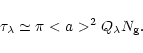
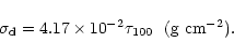
To calculate the mass of dust in GF 17 and GF 20 we calculate the mass column density of dust grains at ![]() m,
m,
![]() ,
as
,
as
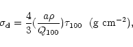 |
(7) |
 |
(8) |
 |
(9) |
Figures 7 and 8 present 13CO integrated emission maps toward GF 17 and GF 20. The molecular gas emission is not uniformly distributed within the clouds. Instead, the emission is seen to arise in chains of condensations strung along their lengths, in a periodic fashion, giving these clouds an overall highly fragmented appearance. We find a remarkably good agreement between our ![]() m optical depth images and our 13CO integrated emission maps. Our optical depth images of GF 17 and GF 20 reproduce the filamentary morphology seen in our 13CO maps. In particular, we see that the
m optical depth images and our 13CO integrated emission maps. Our optical depth images of GF 17 and GF 20 reproduce the filamentary morphology seen in our 13CO maps. In particular, we see that the ![]() m optical depth and 13CO emission images have identified the dense cores within each cloud with remarkable agreement, suggesting that the gas-to-dust ratio is nearly constant throughout these clouds.
m optical depth and 13CO emission images have identified the dense cores within each cloud with remarkable agreement, suggesting that the gas-to-dust ratio is nearly constant throughout these clouds.
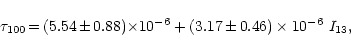
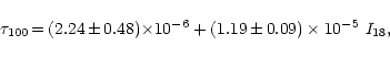
Figure 9 presents a point by point comparison of the ![]() m optical depth and 13CO integrated emission, I13, smoothed to the spatial resolution of IRAS at
m optical depth and 13CO integrated emission, I13, smoothed to the spatial resolution of IRAS at ![]() m, for GF 17 (top) and GF 20 (bottom), respectively. In both cases, filled circles refer to observations toward the filamentary region, and empty circles to observations within the main core region. In the case of GF 17, there is no trend (linear correlation coefficient
m, for GF 17 (top) and GF 20 (bottom), respectively. In both cases, filled circles refer to observations toward the filamentary region, and empty circles to observations within the main core region. In the case of GF 17, there is no trend (linear correlation coefficient ![]() )
of dust
)
of dust ![]() m optical depth with 13CO integrated emission within the main core region. However, we find a strong correlation (
m optical depth with 13CO integrated emission within the main core region. However, we find a strong correlation (![]() )
for the filamentary region. A least-squares fit to the data within this later region yields
)
for the filamentary region. A least-squares fit to the data within this later region yields
 |
(10) |
 |
(11) |
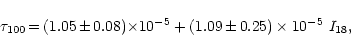
A point by point comparison of the ![]() m optical depth and C18O integrated intensity, I18, smoothed to the spatial resolution of IRAS at
m optical depth and C18O integrated intensity, I18, smoothed to the spatial resolution of IRAS at ![]() m, is shown in Fig. 10. For GF 17, the
m, is shown in Fig. 10. For GF 17, the ![]() m optical depth clearly increases with increasing C18O integrated intensity. Considering all data points, we find a very strong correlation between these two quantities. A least-squares fit yields
m optical depth clearly increases with increasing C18O integrated intensity. Considering all data points, we find a very strong correlation between these two quantities. A least-squares fit yields
 |
(12) |
 |
(13) |
While the dust column density (essentially given by the dust 100 ![]() m optical depth) only traces the depth of dust emission, the gas column density (given by the C18O integrated intensity) is the true value for the clouds, since the tracer molecule is optically thin. However, the fact that the dust column density is well correlated with the gas column density throughout GF 17 and GF 20 implies that the grains responsible for the 60 and 100
m optical depth) only traces the depth of dust emission, the gas column density (given by the C18O integrated intensity) is the true value for the clouds, since the tracer molecule is optically thin. However, the fact that the dust column density is well correlated with the gas column density throughout GF 17 and GF 20 implies that the grains responsible for the 60 and 100 ![]() m emission are well mixed with the gas and are heated by a radiation field that impinges these clouds in a relatively uniform fashion. The morphological similarities between the 100
m emission are well mixed with the gas and are heated by a radiation field that impinges these clouds in a relatively uniform fashion. The morphological similarities between the 100 ![]() m optical depth images and the C18O integrated maps (Moreira & Yun 2002) of GF 17 and GF 20 support this idea. The good agreement between dust optical depth and C18O integrated emission in GF 17 and GF 20 then suggests that the infrared emission must originate from a substantial depth in the clouds. This is consistent with the globular nature of GF 17 and GF 20, where we expect the individual dense cores, connected by lower density material, to be more easily exposed to the local radiation field.
m optical depth images and the C18O integrated maps (Moreira & Yun 2002) of GF 17 and GF 20 support this idea. The good agreement between dust optical depth and C18O integrated emission in GF 17 and GF 20 then suggests that the infrared emission must originate from a substantial depth in the clouds. This is consistent with the globular nature of GF 17 and GF 20, where we expect the individual dense cores, connected by lower density material, to be more easily exposed to the local radiation field.
We thus conclude that far-infrared dust emission can reliably be used as a gas column density tracer in GF 17 and GF 20.
A point by point comparison of the dust temperature and gas column density in GF 17 and GF 20 is shown in Fig. 11 revealing an anticorrelation between these two quantities. The spatial resolutions of both data sets were degraded to match the IRAS ![]() m beam size. The temperature of the dust varies from 33 to 51 K in GF 17, and from 31 to 42 K in GF 20. Hence, the emitting dust in both clouds is substantially hotter than the gas. However, one must be cautious in interpreting these results, since, as noted above, the derived dust temperature is always weighted toward the warmest dust along the line of sight, and dust as cold as the gas will be overwhelmed by the warmer dust and will be unobservable. This explains the fact that the temperatures we calculate (see Table 1) even in the denser, starless main core regions, are significantly higher than
m beam size. The temperature of the dust varies from 33 to 51 K in GF 17, and from 31 to 42 K in GF 20. Hence, the emitting dust in both clouds is substantially hotter than the gas. However, one must be cautious in interpreting these results, since, as noted above, the derived dust temperature is always weighted toward the warmest dust along the line of sight, and dust as cold as the gas will be overwhelmed by the warmer dust and will be unobservable. This explains the fact that the temperatures we calculate (see Table 1) even in the denser, starless main core regions, are significantly higher than ![]() K, while the true gas temperatures (as derived by the 12CO radiation temperatures) are typically below 20 K. Despite these potential difficulties, we believe that the anticorrelation found between the dust temperature and gas column density implies that the dust is warmest where the column densities are smallest. In fact, from the dust temperature maps of GF 17 and GF 20, it is clear that the hotter dust is located at the edges of the clouds. Thus, we find further evidence for GF 17 and GF 20 being externally heated.
K, while the true gas temperatures (as derived by the 12CO radiation temperatures) are typically below 20 K. Despite these potential difficulties, we believe that the anticorrelation found between the dust temperature and gas column density implies that the dust is warmest where the column densities are smallest. In fact, from the dust temperature maps of GF 17 and GF 20, it is clear that the hotter dust is located at the edges of the clouds. Thus, we find further evidence for GF 17 and GF 20 being externally heated.
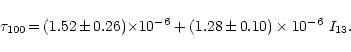
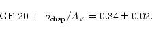
Our calculated dust optical depths toward GF 17 and GF 20 are small, with typical values of
![]() about a factor of 10 smaller than the corresponding values derived by Wood et al. (1994) for 43 nearby molecular clouds. Consequently, small (<1 mag) values of visual extinction (see Table 1) are obtained for GF 17 and GF 20 by means of Eq. (3), and we remind the reader that all extinctions quoted here are lower limits. In order to estimate the pixel-to-pixel (random) errors in AV in each cloud, we examined about 800 pixels within a circular area which appears to have a constant extinction, and obtained a standard deviation in the extinction value of this region of 0.02 mag for both clouds. We use these values as an estimate of the pixel-to-pixel errors in AV, but we remind the reader that this error does not include any errors caused by assuming a constant
about a factor of 10 smaller than the corresponding values derived by Wood et al. (1994) for 43 nearby molecular clouds. Consequently, small (<1 mag) values of visual extinction (see Table 1) are obtained for GF 17 and GF 20 by means of Eq. (3), and we remind the reader that all extinctions quoted here are lower limits. In order to estimate the pixel-to-pixel (random) errors in AV in each cloud, we examined about 800 pixels within a circular area which appears to have a constant extinction, and obtained a standard deviation in the extinction value of this region of 0.02 mag for both clouds. We use these values as an estimate of the pixel-to-pixel errors in AV, but we remind the reader that this error does not include any errors caused by assuming a constant ![]() .
.
Lada et al. (1994) showed that the relation between
![]() ,
the dispersion of extinction measurements within a square map pixel, and AV, the mean extinction derived for the map pixel, can be used to characterize cloud structure on scales smaller than the resolution of the map (i.e. the size of the map pixels). In the molecular cloud IC 5146, Lada et al. (1994) and Lada et al. (1999) found that both
,
the dispersion of extinction measurements within a square map pixel, and AV, the mean extinction derived for the map pixel, can be used to characterize cloud structure on scales smaller than the resolution of the map (i.e. the size of the map pixels). In the molecular cloud IC 5146, Lada et al. (1994) and Lada et al. (1999) found that both
![]() and the dispersion in the
and the dispersion in the
![]() -AV relation increased in a systematic fashion with increasing AV. A similar behaviour for the L977 dark cloud was found by Alves et al. (1998). In order to investigate a
-AV relation increased in a systematic fashion with increasing AV. A similar behaviour for the L977 dark cloud was found by Alves et al. (1998). In order to investigate a
![]() -AV relation for GF 17 and GF 20, we used the AV images generated through Eq. (3). In each AV image, we considered square map pixels (each containing about 400 image pixels) with size similar to the IRAS beam size (
-AV relation for GF 17 and GF 20, we used the AV images generated through Eq. (3). In each AV image, we considered square map pixels (each containing about 400 image pixels) with size similar to the IRAS beam size (
![]() )
at 100
)
at 100 ![]() m. A mean extinction and a dispersion within each map pixel were derived. The top panels of Figs. 12 and 13 present the
m. A mean extinction and a dispersion within each map pixel were derived. The top panels of Figs. 12 and 13 present the
![]() -AV relation for the two clouds, at
-AV relation for the two clouds, at
![]() spatial resolution. The same trend observed in IC 5146 and L977 is found for GF 17 and GF 20. Both
spatial resolution. The same trend observed in IC 5146 and L977 is found for GF 17 and GF 20. Both
![]() and the scatter in the
and the scatter in the
![]() -AV relation increase systematically with AV in GF 17 and GF 20. A least-squares fit over the entire data sets returns the slope of the
-AV relation increase systematically with AV in GF 17 and GF 20. A least-squares fit over the entire data sets returns the slope of the
![]() -AV relation given by
-AV relation given by
 |
(15) |
These values are similar to
![]() and
and
![]() found for IC5146 and L977, respectively, by Alves et al. (1998) and Lada et al. (1999), using near-infrared extinction maps at
found for IC5146 and L977, respectively, by Alves et al. (1998) and Lada et al. (1999), using near-infrared extinction maps at
![]() spatial filtering. Since the estimated distance to both L977 and IC5146 is
spatial filtering. Since the estimated distance to both L977 and IC5146 is ![]() pc, their study has a spatial resolution of 0.2 pc. Interestingly, the present IRAS study of GF 17 and GF 20 (at 150 pc) has the same spatial resolution of 0.2 pc. Hence, we are probing structures with similar physical sizes. Also interesting is the fact that from figure 9 of Lada et al. (1999) we note that for extinctions below a few magnitudes (say less than 5 mag) their
pc, their study has a spatial resolution of 0.2 pc. Interestingly, the present IRAS study of GF 17 and GF 20 (at 150 pc) has the same spatial resolution of 0.2 pc. Hence, we are probing structures with similar physical sizes. Also interesting is the fact that from figure 9 of Lada et al. (1999) we note that for extinctions below a few magnitudes (say less than 5 mag) their
![]() -AV relation is pure noise, while in our study we are sensitive to structure in the same relation but below AV=1. Thus, the NIR- and IRAS-based techniques seem to be complementary regarding the
-AV relation is pure noise, while in our study we are sensitive to structure in the same relation but below AV=1. Thus, the NIR- and IRAS-based techniques seem to be complementary regarding the
![]() -AV relation.
-AV relation.
Lada et al. (1994) have shown that such a relation between
![]() and AV indicate that significant structure must be present down to scales smaller than the resolution of the extinction maps. Thus, the
and AV indicate that significant structure must be present down to scales smaller than the resolution of the extinction maps. Thus, the
![]() -AV relations for GF 17 and GF 20 seem to imply the presence of small-scale structure in the exctinctions toward these clouds. Recently, Lada et al. (1999) used Monte Carlo simulations to show that the form and slope of the
-AV relations for GF 17 and GF 20 seem to imply the presence of small-scale structure in the exctinctions toward these clouds. Recently, Lada et al. (1999) used Monte Carlo simulations to show that the form and slope of the
![]() -AV relation, and hence most (if not all) of the small-scale variations in the extinction, are due to unresolved gradients in the dust distribution within IC 5146 and L977. That is to say that smoothly varying density gradients can produce the "fluctuations'' observed in extinction studies of filamentary clouds. Although (1997) found that the form of the observed
-AV relation, and hence most (if not all) of the small-scale variations in the extinction, are due to unresolved gradients in the dust distribution within IC 5146 and L977. That is to say that smoothly varying density gradients can produce the "fluctuations'' observed in extinction studies of filamentary clouds. Although (1997) found that the form of the observed
![]() versus AV relation in IC5146 is consistent with cloud structure models characterized by supersonic random motions, Lada et al. (1999) note that random spatial fluctuations in the dust distribution could exist (Thoraval et al. 1997), but at a very low level (
versus AV relation in IC5146 is consistent with cloud structure models characterized by supersonic random motions, Lada et al. (1999) note that random spatial fluctuations in the dust distribution could exist (Thoraval et al. 1997), but at a very low level (
![]() at
at
![]() mag), in addition to the smooth gradients.
mag), in addition to the smooth gradients.
Consider Figs. 12 and 13 (bottom panels), where we plot the
![]() -AV relation for both GF 17 and GF 20, but using a spatial filter with angular resolution of
-AV relation for both GF 17 and GF 20, but using a spatial filter with angular resolution of
![]() ,
i.e. half the IRAS beamsize at
,
i.e. half the IRAS beamsize at ![]() m. These diagrams show that when the data are sampled with increased spatial resolution, we obtain a decrease in the slope of the
m. These diagrams show that when the data are sampled with increased spatial resolution, we obtain a decrease in the slope of the
![]() -AV relation. Also, note that the trend of
-AV relation. Also, note that the trend of
![]() increasing with Av appears to be independent of angular resolution. This suggests that structural variations in GF 17 and GF 20 are being increasingly resolved out with higher angular resolution. An identical behaviour was found in IC 5146 by Lada et al. (1999), who argue that such behaviour can be accounted for by a smooth, radially decreasing density gradient of the form
increasing with Av appears to be independent of angular resolution. This suggests that structural variations in GF 17 and GF 20 are being increasingly resolved out with higher angular resolution. An identical behaviour was found in IC 5146 by Lada et al. (1999), who argue that such behaviour can be accounted for by a smooth, radially decreasing density gradient of the form
![]() ,
from 0 to
,
from 0 to ![]() mag of visual extinction. In this context, since we are biased toward low (Av<1 mag) extinctions, we conclude that the edges of GF 17 and GF 20 are likely to be characterized by a similar smooth density gradient. An investigation is underway on the modelling of the internal structures of GF 17 and GF 20 as self-gravitating cylindrical polytropes, and we defer such discussion to a future paper.
mag of visual extinction. In this context, since we are biased toward low (Av<1 mag) extinctions, we conclude that the edges of GF 17 and GF 20 are likely to be characterized by a similar smooth density gradient. An investigation is underway on the modelling of the internal structures of GF 17 and GF 20 as self-gravitating cylindrical polytropes, and we defer such discussion to a future paper.
One of the new phenomena discovered by the IRAS mission is the extensive diffuse infrared emission, strongest at ![]() m, which has become known as the infrared cirrus. These highly structured extended sources are seen predominantly, but not exclusively, at 60 and 100
m, which has become known as the infrared cirrus. These highly structured extended sources are seen predominantly, but not exclusively, at 60 and 100 ![]() m and may originate either in the interplanetary medium, the outer solar system, or the interstellar medium. The infrared cirrus have typical visual extinctions of
m and may originate either in the interplanetary medium, the outer solar system, or the interstellar medium. The infrared cirrus have typical visual extinctions of ![]() mag or less and
mag or less and ![]() m opacities in the range
m opacities in the range
![]() (Low et al. 1984). Several studies (Blitz et al. 1984; Weiland et al. 1986; de Vries et al. 1987) have shown that molecular clouds have been found to be associated with infrared cirrus. Thus, it is of interest to compare the far-infrared emission from GF 17 and GF 20 with the more diffuse infrared cirrus clouds. The most useful means of comparison of these clouds is through the ratio of the 100
(Low et al. 1984). Several studies (Blitz et al. 1984; Weiland et al. 1986; de Vries et al. 1987) have shown that molecular clouds have been found to be associated with infrared cirrus. Thus, it is of interest to compare the far-infrared emission from GF 17 and GF 20 with the more diffuse infrared cirrus clouds. The most useful means of comparison of these clouds is through the ratio of the 100 ![]() m intensity, I100, versus the column density of hydrogen atoms,
m intensity, I100, versus the column density of hydrogen atoms, ![]() .
In the cirrus clouds, Low et al. (1984) derived values of
.
In the cirrus clouds, Low et al. (1984) derived values of
![]() in the range 0.9-2.8 MJy sr
in the range 0.9-2.8 MJy sr
![]() .
Other values of
.
Other values of
![]() of 0.4 to 1.4 MJy sr
of 0.4 to 1.4 MJy sr
![]() were derived by Boulanger et al. (1985), Terebey & Fich (1986), and Boulanger & Perault (1988). Values of
were derived by Boulanger et al. (1985), Terebey & Fich (1986), and Boulanger & Perault (1988). Values of
![]() as high as 1.9 MJy sr
as high as 1.9 MJy sr
![]() have been found for a number of molecular clouds (Boulanger 1989).
have been found for a number of molecular clouds (Boulanger 1989).
Plots of the 100 ![]() m intensity versus molecular hydrogen column density in the edges (i.e., at those locations where the visual extinction is less than say
m intensity versus molecular hydrogen column density in the edges (i.e., at those locations where the visual extinction is less than say ![]() mag) of GF 17 and GF 20 are shown in Fig. 14. The spatial resolutions of both data sets were smoothed to the IRAS beam size at
mag) of GF 17 and GF 20 are shown in Fig. 14. The spatial resolutions of both data sets were smoothed to the IRAS beam size at ![]() m. We note that the 100
m. We note that the 100 ![]() m intensity follows closely (correlation coefficient of
m intensity follows closely (correlation coefficient of ![]() )
the gas column density in the vicinity of GF 17, whereas a rather poor linear trend (
)
the gas column density in the vicinity of GF 17, whereas a rather poor linear trend (![]() )
is seen for GF 20. From the least-squares fits of I100 versus
)
is seen for GF 20. From the least-squares fits of I100 versus
![]() shown in Fig. 14, we have computed the ratio of
shown in Fig. 14, we have computed the ratio of ![]() m intensity to total molecular hydrogen column density, and we obtain 1.78 and 0.76 MJy sr-1 per
m intensity to total molecular hydrogen column density, and we obtain 1.78 and 0.76 MJy sr-1 per
![]() at the edges of GF 17 and GF 20, respectively. Following Snell et al. (1989), we express these ratios in terms of hydrogen atoms to find values of 0.09 and 0.04 MJy sr-1 per
at the edges of GF 17 and GF 20, respectively. Following Snell et al. (1989), we express these ratios in terms of hydrogen atoms to find values of 0.09 and 0.04 MJy sr-1 per
![]() for GF 17 and GF 20, respectively. These values are in excellent agreement with the results for B18 (0.07 MJy sr
for GF 17 and GF 20, respectively. These values are in excellent agreement with the results for B18 (0.07 MJy sr
![]() ), and significantly smaller than those found for the cirrus clouds. Hence, our clouds have lower emission per hydrogen atom than the cirrus clouds.
), and significantly smaller than those found for the cirrus clouds. Hence, our clouds have lower emission per hydrogen atom than the cirrus clouds.
One can also compare the ratio of 60 to ![]() m intensity in our clouds with that found for the cirrus clouds. Low et al. (1984) and Terebey & Fich (1986) obtained an average
I60/I100 ratio of 0.20 for the cirrus clouds. In GF 17 and GF 20, we find a systematic decrease of the
I60/I100 ratio from the edges (
m intensity in our clouds with that found for the cirrus clouds. Low et al. (1984) and Terebey & Fich (1986) obtained an average
I60/I100 ratio of 0.20 for the cirrus clouds. In GF 17 and GF 20, we find a systematic decrease of the
I60/I100 ratio from the edges (
![]() )
to the center of the clouds (
)
to the center of the clouds (
![]() ). Thus, it seems that GF 17 and GF 20 have similar
I60/I100 average ratios, and comparable to the corresponding ratio found in cirrus clouds. This is somewhat unexpected because due to their low visual extinctions (
). Thus, it seems that GF 17 and GF 20 have similar
I60/I100 average ratios, and comparable to the corresponding ratio found in cirrus clouds. This is somewhat unexpected because due to their low visual extinctions (![]() 0.07-0.18 mag, Low et al. 1984, the dust in cirrus clouds can be heated to temperatures significantly larger than the typical IRAS dust temperatures (20-25 K) observed in the inner regions of cold dark clouds (Wood et al. 1994). Therefore, the
I60/I100 ratio appears to be somewhat enhanced in GF 17 and GF 20. However, while the
0.07-0.18 mag, Low et al. 1984, the dust in cirrus clouds can be heated to temperatures significantly larger than the typical IRAS dust temperatures (20-25 K) observed in the inner regions of cold dark clouds (Wood et al. 1994). Therefore, the
I60/I100 ratio appears to be somewhat enhanced in GF 17 and GF 20. However, while the ![]() m emission comes from large dust grains in equilibrium with the radiation field, part of the
m emission comes from large dust grains in equilibrium with the radiation field, part of the ![]() m emission may arise from transiently excited particles (Puget & Léger 1989). Hence, we can interpret our enhanced
I60/I100 ratios in GF 17 and GF 20 as the result of an excitation effect where small grains absorb mainly in the UV and consequently are heated only in a shell at the surfaces of GF 17 and GF 20. This is consistent with the fact that our clouds have (1) comparable peak brightness at either 60 or
m emission may arise from transiently excited particles (Puget & Léger 1989). Hence, we can interpret our enhanced
I60/I100 ratios in GF 17 and GF 20 as the result of an excitation effect where small grains absorb mainly in the UV and consequently are heated only in a shell at the surfaces of GF 17 and GF 20. This is consistent with the fact that our clouds have (1) comparable peak brightness at either 60 or ![]() m, (2) similar 60-100
m, (2) similar 60-100 ![]() m colors, as given by the
I60/I100 ratios, and (3) similar color morphology, in the sense that they exhibit systematic color variations correlated with the opacity (a decrease by a factor of 2 to 3 from the edges to the center).
m colors, as given by the
I60/I100 ratios, and (3) similar color morphology, in the sense that they exhibit systematic color variations correlated with the opacity (a decrease by a factor of 2 to 3 from the edges to the center).
Though the IRAS 60 and 100 ![]() m bands do not detect the emission from most of the dust in these clouds, these bands do include most of the far-infrared luminosity. We can estimate the total far-infrared luminosities of GF 17 and GF 20 from the
m bands do not detect the emission from most of the dust in these clouds, these bands do include most of the far-infrared luminosity. We can estimate the total far-infrared luminosities of GF 17 and GF 20 from the ![]() m and
m and ![]() m images using
m images using
 |
(16) |
The kinematics of a molecular cloud reflects the motions which brought the gas to its current configuration, and can be used to characterize the cloud's evolution. Kinematic signatures in a cloud can result from a variety of phenomena like expanding H II regions, powerfull stellar winds, supernova explosions, outflows, magnetic fields, or even from simple solid-body rotation or galactic shear. For example, the morphology of the ![]() Oph complex (Vrba 1977; Loren 1989) suggests that both shocks and magnetic fields are the main mechanisms responsible for the elongation of the dark clouds L1709, L1755, L1729, and L1689N. These clouds are long filaments extending from the star-forming cores in
Oph complex (Vrba 1977; Loren 1989) suggests that both shocks and magnetic fields are the main mechanisms responsible for the elongation of the dark clouds L1709, L1755, L1729, and L1689N. These clouds are long filaments extending from the star-forming cores in ![]() Oph, and are aligned along a direction pointing toward the Upper-Scorpius (hereafter USco) subgroup of the Sco OB2 association (Loren 1989). External forces, such as an expanding supernova remnant or H II shell, applied to a gas complex can accelerate different clump masses at different rates. Differential acceleration can stretch a cloud into an elongated filament with the most massive component closest to the source of the external force. As a result, a velocity gradient is expected to appear along the filament axis. On the other hand, if different mass elements along a filament's length have the same
Oph, and are aligned along a direction pointing toward the Upper-Scorpius (hereafter USco) subgroup of the Sco OB2 association (Loren 1989). External forces, such as an expanding supernova remnant or H II shell, applied to a gas complex can accelerate different clump masses at different rates. Differential acceleration can stretch a cloud into an elongated filament with the most massive component closest to the source of the external force. As a result, a velocity gradient is expected to appear along the filament axis. On the other hand, if different mass elements along a filament's length have the same
![]() ,
then it is evidence for there being no component of external force along the line of sight. Finally, while any differences in
,
then it is evidence for there being no component of external force along the line of sight. Finally, while any differences in
![]() from one end of a filament to the other are most likely not the result of rotation, transverse gradients are more likely to be the result of large-scale rotation (Goodman et al. 1993). Thus, studies of the velocity fields within molecular clouds are of crucial importance in order to characterize the dynamical state of the clouds.
from one end of a filament to the other are most likely not the result of rotation, transverse gradients are more likely to be the result of large-scale rotation (Goodman et al. 1993). Thus, studies of the velocity fields within molecular clouds are of crucial importance in order to characterize the dynamical state of the clouds.
The extensive velocity information contained in spectral-line maps provides the opportunity to analyse motions in molecular clouds carefully, and thus to estimate accurately the magnitude and direction of the velocity gradients, if present. The CO and 13CO lines are a useful probe of the large-scale velocity field in a cloud because of its widespread detectability, but are not an unbiased probe in all cases, due to opacity effects. In the case of GF 20, we have decided to use the CO line as a probe because the lines are gaussian in shape and narrow (
![]() km s-1). For GF 17, we selected the 13CO line because the CO line was found to be very assymetric and broad (
km s-1). For GF 17, we selected the 13CO line because the CO line was found to be very assymetric and broad (
![]() km s-1) toward most lines-of-sight. Nevertheless, it is extremely unlikely that our velocity gradient calculations will be significantly affected by opacity effects because narrow linewidths do not allow large errors in velocity, even for lines-of-sight with large optical depths. Although available for fewer positions, the C18O data was also used to probe the kinematic signatures that may exist within the denser regions.
km s-1) toward most lines-of-sight. Nevertheless, it is extremely unlikely that our velocity gradient calculations will be significantly affected by opacity effects because narrow linewidths do not allow large errors in velocity, even for lines-of-sight with large optical depths. Although available for fewer positions, the C18O data was also used to probe the kinematic signatures that may exist within the denser regions.
In Fig. 15, the LSR central velocity of the 13CO (GF 17) and CO (GF 20) lines is plotted against right ascension offset from the reference map positions. The velocity resolutions are 0.12 km s-1 for CO (in GF 17) and 0.11 km s-1 for 13CO (in GF 20). The vertical dashed lines separate the main core region from the filamentary region in each cloud. A striking dependence (over
![]() in right ascension offset in both clouds) of line velocity with position is clearly seen. We focus our analysis on the following remarks:
in right ascension offset in both clouds) of line velocity with position is clearly seen. We focus our analysis on the following remarks:
If the cloud producing the emission line rotates as a solid body,
![]() will be independent of distance along the line of sight, and linearly dependent on the coordinates in the plane of the sky (Goodman et al. 1993). Thus a cloud undergoing solid-body rotation can be expected to exhibit a linear gradient,
will be independent of distance along the line of sight, and linearly dependent on the coordinates in the plane of the sky (Goodman et al. 1993). Thus a cloud undergoing solid-body rotation can be expected to exhibit a linear gradient,
![]() ,
across the face of a map, perpendicular to the rotation axis. We fit the function
,
across the face of a map, perpendicular to the rotation axis. We fit the function
![]() to the data, where
to the data, where
![]() and
and
![]() represent offsets in right ascension and declination, expressed in radians, a and b are the projections of the gradient per radian on the
represent offsets in right ascension and declination, expressed in radians, a and b are the projections of the gradient per radian on the ![]() and
and ![]() axes, and V0 is the systemic velocity of the cloud, with respect to the local standard of rest. The magnitude of the velocity gradient, in a cloud at distance D, is then given by
axes, and V0 is the systemic velocity of the cloud, with respect to the local standard of rest. The magnitude of the velocity gradient, in a cloud at distance D, is then given by
![]() and its direction (the direction of increasing velocity, measured east of north) is given by
and its direction (the direction of increasing velocity, measured east of north) is given by
![]() .
From this, we can estimate the amount of solid-body rotation implied by the observed line of sight velocity field in a cloud. However, note that rotation is only one possible interpretation for any gradient found.
.
From this, we can estimate the amount of solid-body rotation implied by the observed line of sight velocity field in a cloud. However, note that rotation is only one possible interpretation for any gradient found.
We have used the routine by Goodman et al. (1993), which performs a least-squares fit to the velocity field observed in a spectral-line map of a molecular cloud, and returns the magnitude of the gradient, its direction, and the errors in those quantities. Each observed value of
![]() is weighted by
is weighted by
![]() ,
where
,
where
![]() is the uncertainty in
is the uncertainty in
![]() determined by a Gaussian fit to the line profile. Fitting all 13CO data points in GF 17, we find a best-fit velocity gradient of
determined by a Gaussian fit to the line profile. Fitting all 13CO data points in GF 17, we find a best-fit velocity gradient of
![]() km s-1 pc-1 with direction
km s-1 pc-1 with direction
![]() east of north; fitting all the C18O data, one obtains the same magnitude for the best-fit velocity gradient and a slightly different direction,
east of north; fitting all the C18O data, one obtains the same magnitude for the best-fit velocity gradient and a slightly different direction,
![]() .
For GF 20, the CO best-fit velocity gradient is
.
For GF 20, the CO best-fit velocity gradient is ![]() km s-1 pc-1 with direction
km s-1 pc-1 with direction
![]() ,
again in good agreement with the values derived from all the C18O data (
,
again in good agreement with the values derived from all the C18O data (
![]() km s-1 pc-1 and
km s-1 pc-1 and
![]() ). To estimate the significance of our derived velocity gradients, we calculate the ratio
). To estimate the significance of our derived velocity gradients, we calculate the ratio
![]() ,
where
,
where ![]() is the error in the fitted velocity gradient. We find ratios of 267 and 16 for 13CO and C18O, respectively, in GF 17, and 667 and 24 for CO and C18O, respectively, in GF 20. Thus, our best-fit velocity gradients are very robust.
is the error in the fitted velocity gradient. We find ratios of 267 and 16 for 13CO and C18O, respectively, in GF 17, and 667 and 24 for CO and C18O, respectively, in GF 20. Thus, our best-fit velocity gradients are very robust.
Considering the plane-of-the-sky orientation of GF 20, we conclude that the overall velocity gradients found are roughly perpendicular to the major axis of the filamentary structure. In principle, this could be interpreted as large-scale rotation of the cloud about its major axis. However, in this case a linear dependence of
![]() along the full extent of the cloud would be expected. As shown in Fig. 15, this is not the case since the sense of the increase in
along the full extent of the cloud would be expected. As shown in Fig. 15, this is not the case since the sense of the increase in
![]() within the main core region does not coincide with that found for the filamentary region. To better analyze the kinematic differences between the filamentary regions and the main core regions of GF 17 and GF20, we have calculated best-fit velocity gradients within those regions separately. The results are listed in Table 2. Clearly, the velocity gradients within the main core regions and those within the filamentary regions exhibit different plane-of-the-sky orientations, but also differ in magnitude (typically a factor 2-2.5 larger in the main core regions). Caution should be taken in interpreting the velocity shifts in the main core regions as simple streaming motions, because as mentioned above (1) these regions exhibit possibly several blended velocity components, and (2) the observed changes in velocity in those regions are comparable or smaller than the CO and 13CO line widths therein, suggesting that we may be witnessing changes in the relative strength of different components along the line of sight. In any case, comparing the filamentary regions or the main core regions in both clouds, we find very similar magnitudes of the best-fit velocity gradients. We also note that the directions of the best-fit velocity gradients in the main core regions are remarkably similar. Taken together, these results argue that simple large-scale rotation cannot account for the velocity gradients and their similarities in GF 17 and GF 20, and instead strongly suggest a more complex, common origin.
within the main core region does not coincide with that found for the filamentary region. To better analyze the kinematic differences between the filamentary regions and the main core regions of GF 17 and GF20, we have calculated best-fit velocity gradients within those regions separately. The results are listed in Table 2. Clearly, the velocity gradients within the main core regions and those within the filamentary regions exhibit different plane-of-the-sky orientations, but also differ in magnitude (typically a factor 2-2.5 larger in the main core regions). Caution should be taken in interpreting the velocity shifts in the main core regions as simple streaming motions, because as mentioned above (1) these regions exhibit possibly several blended velocity components, and (2) the observed changes in velocity in those regions are comparable or smaller than the CO and 13CO line widths therein, suggesting that we may be witnessing changes in the relative strength of different components along the line of sight. In any case, comparing the filamentary regions or the main core regions in both clouds, we find very similar magnitudes of the best-fit velocity gradients. We also note that the directions of the best-fit velocity gradients in the main core regions are remarkably similar. Taken together, these results argue that simple large-scale rotation cannot account for the velocity gradients and their similarities in GF 17 and GF 20, and instead strongly suggest a more complex, common origin.
| Cloud | Region | Gradient | Direction | Gradient | Number of | Region |
| (km s-1 pc-1) | (deg E of N) | significance | points in fit | of fit | ||
| CO | ||||||
| GF 20 | filament | 0.48 | 40 | 180 | 397 |
|
| main core | 1.22 | -83 | 392 | 132 |
|
|
| 13CO | ||||||
| GF 17 | filament | 0.39 | 94 | 288 | 288 |
|
| main core | 0.80 | -80 | 47 | 80 |
|
|
| C18O | ||||||
| GF 17 | filament | 0.66 | 63 | 23 | 108 |
|
| main core | 1.63 | -132 | 21 | 26 |
|
|
| GF 20 | filament | 0.30 | 153 | 7 | 264 |
|
| main core | 2.29 | -157 | 9 | 9 |
|
|
Could galactic shear produce such velocity gradients? It seems very unlikely because the overall best-fit velocity gradients in GF 17 and GF 20 given above are nearly perpendicular to the galactic plane. Still, we can estimate the inclination to the plane of the sky of GF 17 and GF 20 which is required so that the velocity gradient induced by galactic shear reproduces the velocity gradients observed. The velocity gradient induced in a cloud with galactic longitude, l, at an inclination angle, i, to the plane-of-the-sky is given by
![]() tan(i)
tan(i)![]() ,
where A is the Oort A constant and
,
where A is the Oort A constant and ![]() is the offset position across the face of the cloud map. From Fig. 15 we take
is the offset position across the face of the cloud map. From Fig. 15 we take
![]() km s-1, corresponding to the velocity shift observed across
km s-1, corresponding to the velocity shift observed across
![]() (or about
(or about
![]() pc) along the filamentary regions of GF 17 or GF 20. Using A=16 km s-1 kpc-1 (Mihalas & Binney 1981), we derive
pc) along the filamentary regions of GF 17 or GF 20. Using A=16 km s-1 kpc-1 (Mihalas & Binney 1981), we derive
![]() .
Then, if galactic shear is the dominant mechanism producing the observed velocity gradient, this requires that GF 17 and GF 20 be nearly perpendicular to the plane-of-the-sky, i.e. along the line-of-sight. This seems very unlikely because it would imply that the true extent of the filamentary regions in GF 17 and GF 20 would have to be of the order of
.
Then, if galactic shear is the dominant mechanism producing the observed velocity gradient, this requires that GF 17 and GF 20 be nearly perpendicular to the plane-of-the-sky, i.e. along the line-of-sight. This seems very unlikely because it would imply that the true extent of the filamentary regions in GF 17 and GF 20 would have to be of the order of ![]() pc, that is to say of the order of the diameter of the whole Lupus complex of dark clouds. Furthermore, these clouds appear to be small and dense, and thus insusceptible to the effects of a differential gravitational field. Thus, the velocity structures of GF 17 and GF 20 were likely produced by some mechanism other than galactic shear or simple large-scale rotation. We discuss the nature of such mechanism in Sect. 5.2.
pc, that is to say of the order of the diameter of the whole Lupus complex of dark clouds. Furthermore, these clouds appear to be small and dense, and thus insusceptible to the effects of a differential gravitational field. Thus, the velocity structures of GF 17 and GF 20 were likely produced by some mechanism other than galactic shear or simple large-scale rotation. We discuss the nature of such mechanism in Sect. 5.2.
Copyright ESO 2002
![\begin{figure}
\par\includegraphics[width=18cm,clip]{ms1437f3.eps}\end{figure}](/articles/aa/full/2002/02/aa1437/img93.gif)
![\begin{figure}
\par\includegraphics[width=18cm,clip]{ms1437f4.eps}\end{figure}](/articles/aa/full/2002/02/aa1437/img94.gif)
![\begin{figure}
\par\includegraphics[width=13.5cm,clip]{ms1437f5.eps}\end{figure}](/articles/aa/full/2002/02/aa1437/img108.gif)
![\begin{figure}
\par\includegraphics[width=13.5cm,clip]{ms1437f6.eps}\end{figure}](/articles/aa/full/2002/02/aa1437/img109.gif)
![\begin{figure}
\par\includegraphics[width=13cm,clip]{ms1437f7.eps} %
\end{figure}](/articles/aa/full/2002/02/aa1437/img129.gif)
![\begin{figure}
\par\includegraphics[angle=-90,width=12cm,clip]{ms1437f8.eps} %
\end{figure}](/articles/aa/full/2002/02/aa1437/img130.gif)
![\begin{figure}
\par\includegraphics[width=10cm,clip]{ms1437f9.eps}\end{figure}](/articles/aa/full/2002/02/aa1437/img133.gif)
![\begin{figure}
\par\includegraphics[width=10cm,clip]{ms1437f10.eps} %
\end{figure}](/articles/aa/full/2002/02/aa1437/img138.gif)
![\begin{figure}
\par\includegraphics[width=8.8cm,clip]{ms1437f11.eps}\end{figure}](/articles/aa/full/2002/02/aa1437/img141.gif)
![\begin{figure}
\par\includegraphics[width=8.8cm,clip]{ms1437f12.eps}\end{figure}](/articles/aa/full/2002/02/aa1437/img149.gif)
![\begin{figure}
\par\includegraphics[width=8.8cm,clip]{ms1437f13.eps}\end{figure}](/articles/aa/full/2002/02/aa1437/img150.gif)
![\begin{figure}
\par\includegraphics[angle=-90,width=18cm,clip]{ms1437f14.eps}\end{figure}](/articles/aa/full/2002/02/aa1437/img165.gif)
![\begin{figure}
\par\includegraphics[angle=-90,width=18cm,clip]{ms1437f15.eps}\end{figure}](/articles/aa/full/2002/02/aa1437/img183.gif)