The 60 and 100 ![]() m dust color temperature,
m dust color temperature, ![]() ,
was calculated at each pixel in an image assuming that the dust in a single beam can be characterized by one single temperature (
,
was calculated at each pixel in an image assuming that the dust in a single beam can be characterized by one single temperature (![]() ), and that the emission at 60 and 100
), and that the emission at 60 and 100 ![]() m is due to blackbody radiation from dust grains at temperature
m is due to blackbody radiation from dust grains at temperature ![]() ,
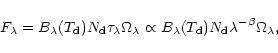
modified by a power-law emissivity. The flux density of optically thin emission from dust grains at wavelength
,
modified by a power-law emissivity. The flux density of optically thin emission from dust grains at wavelength ![]() is given by (e.g. Arce & Goodman 1999)
is given by (e.g. Arce & Goodman 1999)
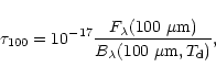
Assuming optically thin emission, we use the dust color temperature to calculate the dust optical depth at each pixel
In order to derive the dust temperature and optical depths, we have made the following assumptions: (1) the dust is optically thin at 60 and 100 ![]() m, (2) dust emissivity is proportional to a power law
m, (2) dust emissivity is proportional to a power law
![]() ,
with index
,
with index ![]() ,
and (3) the dust in the IRAS beam is at a single temperature. We discuss the validity of these assumptions below.
,
and (3) the dust in the IRAS beam is at a single temperature. We discuss the validity of these assumptions below.
Draine & Lee (1984) have shown that the ![]() m optical depth can be estimated in terms of the hydrogen column density along the line of sight as
m optical depth can be estimated in terms of the hydrogen column density along the line of sight as
![]() .
Thus,
.
Thus,
![]() only for
only for ![]() in excess of
in excess of
![]() cm-2, which is well above typical Galactic plane values. In addition, the largest
cm-2, which is well above typical Galactic plane values. In addition, the largest
![]() we find in our images is
we find in our images is
![]() .
Thus, assumption (1) is valid.
.
Thus, assumption (1) is valid.
The errors introduced by assuming a constant ![]() along the line of sight are hard to estimate, since we do not have any way to measure how much
along the line of sight are hard to estimate, since we do not have any way to measure how much ![]() changes in our regions of study. There is a general agreement that the emissivity index depends on the grain size, composition, and physical structure (Weintraub et al. 1991), and the general consensus in recent years has been that
changes in our regions of study. There is a general agreement that the emissivity index depends on the grain size, composition, and physical structure (Weintraub et al. 1991), and the general consensus in recent years has been that ![]() has a value most likely between 1 and 2, that in the general ISM
has a value most likely between 1 and 2, that in the general ISM ![]() is close to 2, and in denser regions with bigger grains
is close to 2, and in denser regions with bigger grains ![]() is closer to 1 (Beckwith & Sargent 1991; Mannings & Emerson 1994; Pollack et al. 1994). We have performed tests with
is closer to 1 (Beckwith & Sargent 1991; Mannings & Emerson 1994; Pollack et al. 1994). We have performed tests with ![]() and find that our results are not significantly affected: for both clouds, the dust color temperature calculations with
and find that our results are not significantly affected: for both clouds, the dust color temperature calculations with ![]() and
and ![]() are consistent within
are consistent within ![]() .
Thus, we conclude that assumption (2) is acceptable.
.
Thus, we conclude that assumption (2) is acceptable.
Assumption (3) is certainly not valid near local heat sources. Langer et al. (1989) and Draine (1990) have considered this problem by examining a simple two-component model where the two regions have different dust temperatures and optical depths. They have shown that the calculated dust temperature is dominated by the emission from the hot dust component, even if this component represents only a few percent of the total mass of dust. Essentially our temperature determination, from which we calculate the ![]() m and
m and ![]() m emission, is an emissivity weighted rather than a mass weighted dust temperature. Thus, our single-temperature assumption is violated in the immediate vicinity of stars embedded in the cloud. If a star heats the dust in its vicinity, the calculated
T60/100 will be dominated by the hot dust, the derived
m emission, is an emissivity weighted rather than a mass weighted dust temperature. Thus, our single-temperature assumption is violated in the immediate vicinity of stars embedded in the cloud. If a star heats the dust in its vicinity, the calculated
T60/100 will be dominated by the hot dust, the derived
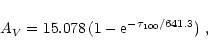
![]() will be too low and consequently AV will be underestimated. Hence, the masses of the clouds that have embedded stars with unresolved dust temperature gradients will also be underestimated. Even away from the point sources, complex temperature structure may be present and must be kept under consideration when interpreting the derived dust optical depths and temperatures. Without higher spatial resolution observations or modeling the dust temperature distribution close to embedded stars we cannot remove this effect.
will be too low and consequently AV will be underestimated. Hence, the masses of the clouds that have embedded stars with unresolved dust temperature gradients will also be underestimated. Even away from the point sources, complex temperature structure may be present and must be kept under consideration when interpreting the derived dust optical depths and temperatures. Without higher spatial resolution observations or modeling the dust temperature distribution close to embedded stars we cannot remove this effect.
In estimating the physical parameters of the molecular gas in GF 17 and GF 20, we have assumed that the main beam temperature,
![]() ,
is a good approximation of the source brightness temperature, since the molecular structures observed are extended with respect to the telescope beam. We assume a plane-parallel, LTE, isothermal, and optically thin radiative transfer model for the 13CO transition line.
,
is a good approximation of the source brightness temperature, since the molecular structures observed are extended with respect to the telescope beam. We assume a plane-parallel, LTE, isothermal, and optically thin radiative transfer model for the 13CO transition line.
The excitation temperature of each line of sight in each cloud was computed from the peak CO intensity under the assumptions of high optical depth of the CO line and a beam-filling factor of unity, using the equation
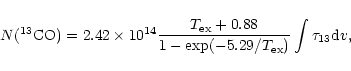
From the 13CO observations, we can obtain the column densities of the cloud with the usual assumptions that (1) CO is optically thick, (2) 13CO is optically thin, (3) the CO and 13CO transitions have the same excitation temperatures, and (4) the same beam filling factor. The optical depth of the 13CO line can be obtained by using the measured temperatures of CO and 13CO at each position toward the cloud:
Combining ![]() and
and
![]() ,
the LTE column density of 13CO can be estimated as (e.g. Bourke et al. 1997)
,
the LTE column density of 13CO can be estimated as (e.g. Bourke et al. 1997)
We derive an estimate of the cloud mass from the 13CO observations by integrating Eq. (6) over the solid angle subtended by the source. For the areas covered by our 13CO maps, we find gas masses of
![]() and
and
![]() for GF 17 and GF 20, respectively, assuming a distance of 150 pc to the Lupus complex. In GF 17, our 13CO maps are limited to a region which is much smaller than the full extent of the cloud. Assuming similar conditions outside the areas covered in this study, the total mass of GF 17 may amount to
for GF 17 and GF 20, respectively, assuming a distance of 150 pc to the Lupus complex. In GF 17, our 13CO maps are limited to a region which is much smaller than the full extent of the cloud. Assuming similar conditions outside the areas covered in this study, the total mass of GF 17 may amount to
![]() ,
in good agreement with the estimate by Andreazza & Vilas-Boas (1996), and we regard this as an upper limit since the density is seen to drop significantly towards the cloud boundaries. On the other hand, GF 20 (which was almost completely mapped) has very low mass, a factor of
,
in good agreement with the estimate by Andreazza & Vilas-Boas (1996), and we regard this as an upper limit since the density is seen to drop significantly towards the cloud boundaries. On the other hand, GF 20 (which was almost completely mapped) has very low mass, a factor of ![]() smaller than the previous estimate by Tachihara et al. (1996).
smaller than the previous estimate by Tachihara et al. (1996).
Copyright ESO 2002
![\begin{displaymath}%
\frac{T_{0}}{T_{\rm ex}}={\rm ln}\left[1+\frac{T_{0}}{J(T_{\rm bg})+T_{\rm mb}}\right],
\end{displaymath}](/articles/aa/full/2002/02/aa1437/img75.gif)
![\begin{displaymath}%
\frac{T_{\rm mb}({\rm CO})}{T_{\rm mb}(^{13}{\rm CO})}\approx \frac{[1-{\rm exp}(-X\tau_{13})]}{[1-{\rm exp}(-\tau_{13})]},
\end{displaymath}](/articles/aa/full/2002/02/aa1437/img80.gif)