As pointed out by Gray & Garrison (1987), there is no "standard'' technique for measuring projected rotational velocity.
The first application of Fourier analysis in the determination of stellar rotational velocities was undertaken by Carroll (1933).
Gray (1992) uses the whole profile of Fourier transform of spectral lines to derive the
![]() ,
instead of only the zeroes as suggested by Carroll.
The
,
instead of only the zeroes as suggested by Carroll.
The
![]() measurement method we adopted is based on the position of
the first zero of the Fourier transform (FT) of the line profiles
(Carroll 1933). The shape of the first lobe of the FT allows us to
better and more easily identify rotation as the main broadening agent of a line compared to the line profile in the wavelength domain. FT of the spectral line is computed using a Fast Fourier Transform algorithm. The
measurement method we adopted is based on the position of
the first zero of the Fourier transform (FT) of the line profiles
(Carroll 1933). The shape of the first lobe of the FT allows us to
better and more easily identify rotation as the main broadening agent of a line compared to the line profile in the wavelength domain. FT of the spectral line is computed using a Fast Fourier Transform algorithm. The
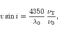
![]() value is derived from the position of the first zero of the FT of the observed line using a theoretical rotation profile for a line at 4350Å and
value is derived from the position of the first zero of the FT of the observed line using a theoretical rotation profile for a line at 4350Å and
![]() equal to 1
equal to 1
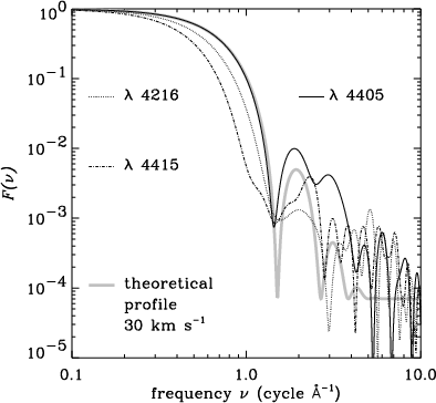
![]() (Ramella et al. 1989). The whole profile in the Fourier domain is then compared with a theoretical rotational profile for the corresponding velocity to check if the first lobes correspond (Fig. 3).
(Ramella et al. 1989). The whole profile in the Fourier domain is then compared with a theoretical rotational profile for the corresponding velocity to check if the first lobes correspond (Fig. 3).
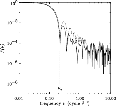 |
Figure 3:
Profile of the Fourier transform of the Mg II 4481Å line (solid line) for the star HIP 95965 and theoretical rotational profile (dashed line) with
|
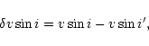
If ![]() is the position of the first zero of the line profile (at
is the position of the first zero of the line profile (at ![]() )
in the Fourier space, the projected rotational velocity is derived as follows:
)
in the Fourier space, the projected rotational velocity is derived as follows:
It should be noted that we did not take into account the gravity darkening, effect that can play a role in rapidly rotating stars when velocity is close to break-up, as this is not relevant for most of our targets.
Determination of the projected rotational velocity requires normalized spectra.
As far as the continuum is concerned, it has been determined visually, passing through noise fluctuations. The MIDAS procedure for continuum determination of 1D-spectra has been used, fitting a spline over the points chosen in the graphs.
Uncertainty related to this determination rises because the continuum observed on the spectrum is a pseudo-continuum. Actually, the true continuum is, in this spectral domain, not really reached for this type of stars.
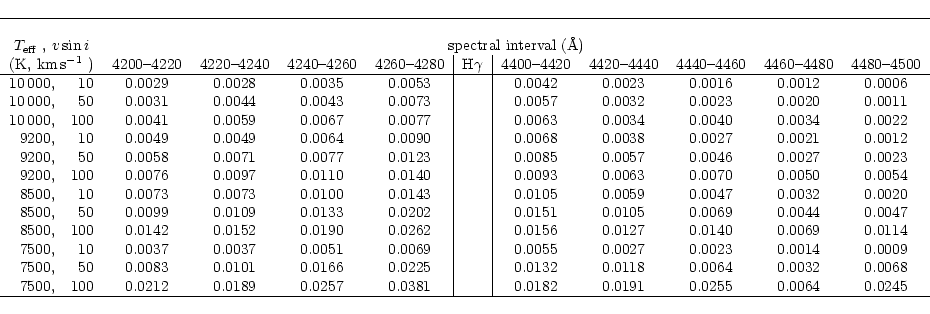
In order to quantify this effect, a grid of synthetic spectra of different effective temperatures (10000, 9200, 8500 and 7500K) and different rotational broadenings has been computed from Kurucz' model atmosphere (Kurucz 1993), and Table 1 lists the differences between the true continuum and the pseudo-continuum represented as the highest points in the spectra.
|
|
Continuum is then tilted to origin and the spectral windows corresponding to lines of interest are extracted from the spectrum in order to compute their FT.
The essential step in this analysis is the search for suitable spectral lines to measure the
![]() .
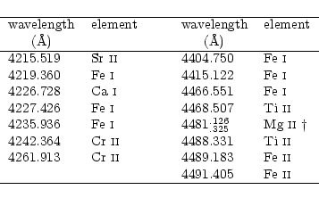
The lines which are candidates for use in the determination of rotation (Table 2) have been identified in the Sirius atlas (Furenlid et al. 1992) and retained according to the following criteria:
.
The lines which are candidates for use in the determination of rotation (Table 2) have been identified in the Sirius atlas (Furenlid et al. 1992) and retained according to the following criteria:
|
|
The lines selected in the Sirius spectrum are valid for early A-type
stars. When moving to stars cooler than about A3-type stars, the effects of
the increasing incidence of blends and the presence of stronger
metallic lines must be taken into account. The effects are: (1) an
increasing departure of the true continuum flux (to which the spectrum
must be normalized) from the curve that joins the highest points in
the observed spectrum, as mentioned in the previous subsection, and (2)
an increased incidence of blending that reduces the number of
lines suitable for
![]() measurements. The former effect will be
estimated in Sect. 3.4. The latter can be derived from the symmetry
of the spectral lines.
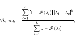
Considering a line, continuum tilted to zero, as a distribution, moments of kth order can be defined as:
measurements. The former effect will be
estimated in Sect. 3.4. The latter can be derived from the symmetry
of the spectral lines.
Considering a line, continuum tilted to zero, as a distribution, moments of kth order can be defined as:
The most noticeable finding in this table is that
![]() usually
increases with decreasing
usually
increases with decreasing
![]() and increasing
and increasing
![]() .
This is a typical effect of blends. Nevertheless, high rotational broadening can lower the skewness of a blended line by making the blend smoother.
.
This is a typical effect of blends. Nevertheless, high rotational broadening can lower the skewness of a blended line by making the blend smoother.
Skewness ![]() for the synthetic spectrum close to Sirius' parameters (
for the synthetic spectrum close to Sirius' parameters (
![]() K,
K,
![]()
![]() )
is contained between -0.09 and +0.10. The threshold, beyond which blends are regarded as affecting the profile significantly, is taken as equal to 0.15. If
)
is contained between -0.09 and +0.10. The threshold, beyond which blends are regarded as affecting the profile significantly, is taken as equal to 0.15. If
![]() the line is not taken into account in the derivation of the
the line is not taken into account in the derivation of the
![]() for a star with corresponding spectral type and rotational broadening. This threshold is a compromise between the unacceptable distortion of the line and the number of retained lines, and it ensures that the differences between centroid and theoretical wavelength of the lines have a standard deviation of about 0.02 Å.
for a star with corresponding spectral type and rotational broadening. This threshold is a compromise between the unacceptable distortion of the line and the number of retained lines, and it ensures that the differences between centroid and theoretical wavelength of the lines have a standard deviation of about 0.02 Å.
As can be expected, moving from B8 to F2-type stars increases the blending of lines. Among the lines listed in Table 2, the strongest ones in Sirius spectrum (Sr II 4216, Fe I 4219, Cr II 4242, Fe I 4405 and Mg II 4481) correspond to those which remain less contaminated by the presence of other lines. Only Fe I 4405 retains a symmetric profile not being heavily blended at the resolution of our spectra and thus measurable all across the grid of the synthetic spectra.
The Mg II doublet at 4481Å is usually chosen to measure
the
![]() :
it is not very sensitive to stellar effective temperature
and gravity and its relative strength in late B through mid-A-type
star spectra makes it almost the only measurable line in this
:
it is not very sensitive to stellar effective temperature
and gravity and its relative strength in late B through mid-A-type
star spectra makes it almost the only measurable line in this
Among the list of candidate lines chosen according to the spectral type and rotational broadening of the star, some can be discarded on the basis of the spectrum quality itself. The main reason for discarding a line, first supposed to be reliable for
![]() determination, lies in its profile in Fourier space. One retains the results given by lines whose profile correspond to a rotational profile.
determination, lies in its profile in Fourier space. One retains the results given by lines whose profile correspond to a rotational profile.
In logarithmic frequency space, such as in Figs. 3 and 5, the rotational profile has a unique shape, and the effect of
![]() simply acts as a translation in frequency. Matching between the theoretical profile, shifted at the ad hoc velocity, and the observed profile, is used as confirmation of the value of the first zero as a
simply acts as a translation in frequency. Matching between the theoretical profile, shifted at the ad hoc velocity, and the observed profile, is used as confirmation of the value of the first zero as a
![]() .
.
A discarded Fourier profile is sometimes associated with a distorted profile in wavelength space, but this is not always the case. For low rotational broadening, i.e.
![]()
![]() ,
the Fourier profile deviates from the theoretical rotational profile. This is due to the fact that rotation does not completely dominate the line profile and the underlying instrumental profile is no longer negligible. It may also occur that an SB2 system, where lines of both components are merged, appears as a single star, but the blend due to multiplicity makes the line profile diverge from a rotational profile.
,
the Fourier profile deviates from the theoretical rotational profile. This is due to the fact that rotation does not completely dominate the line profile and the underlying instrumental profile is no longer negligible. It may also occur that an SB2 system, where lines of both components are merged, appears as a single star, but the blend due to multiplicity makes the line profile diverge from a rotational profile.
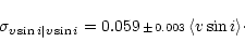
To conclude, the number of measurable lines among the 15 listed in Table 2 also varies from one spectrum to another according to the rotational broadening and the signal-to-noise ratio and ranges from 1 to 15 lines.
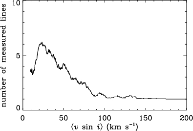 |
Figure 6:
Average number of measured lines (running average over 30 points) is plotted as a function of the mean
|
 |
(5) |
This estimation of the effect of the continuum is only carried out on synthetic spectra because the way our observed spectra have been normalized offers no way to recover the true continuum. The resulting shift is given here for information only.
Two types of uncertainties are present: those internal to the method and those related to the line profile.
The internal error comes from the uncertainty in the real position of the first zero due to the sampling in the Fourier space. The Fourier transforms are computed over 1024 points equally spaced with the step ![]() .
This step is inversely proportional to the step in wavelength space
.
This step is inversely proportional to the step in wavelength space
![]() ,
and the spectra are sampled with
,
and the spectra are sampled with
![]() Å. The uncertainty of
Å. The uncertainty of
![]() due to the sampling is
due to the sampling is
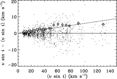
The best way to estimate the precision of our measurements is to study the dispersion of the individual
![]() .
For each star,
.
For each star,
![]() is an average of the individual values derived from selected lines.
is an average of the individual values derived from selected lines.
Residual around this formal error can be expected to depend on the
effective temperature of the star. Figure 9 displays
the variations of the residuals as a function of the spectral
type. Although contents of each bin of spectral type are not constant
all across the sample (the error bar is roughly proportional to the
logarithm of the inverse of the number of points), there does not seem to be
any trend, which suggests that our choice of lines according to the
spectral type eliminates any systematic effect due to the stellar temperature from the measurement
of the
![]() .
.
The differences
![]() ,
normalized by the
formal error
,
normalized by the
formal error
![]() ,
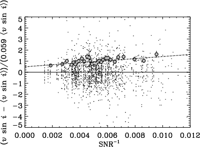
are plotted versus the
noise level (SNR-1) in Fig. 10 in order to
estimate the effect of SNR. Noise is derived for each spectrum using a
piecewise-linear high-pass filter in Fourier space with a transition
band chosen between 0.3 and 0.4 times the Nyquist frequency;
standard deviation of this high frequency signal is computed as the
noise level and then divided by the signal level. The trend in
Fig. 10 is computed as for Fig. 8,
using a robust estimation and GaussFit.
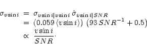
The linear adjustment gives:
,
are plotted versus the
noise level (SNR-1) in Fig. 10 in order to
estimate the effect of SNR. Noise is derived for each spectrum using a
piecewise-linear high-pass filter in Fourier space with a transition
band chosen between 0.3 and 0.4 times the Nyquist frequency;
standard deviation of this high frequency signal is computed as the
noise level and then divided by the signal level. The trend in
Fig. 10 is computed as for Fig. 8,
using a robust estimation and GaussFit.
The linear adjustment gives:
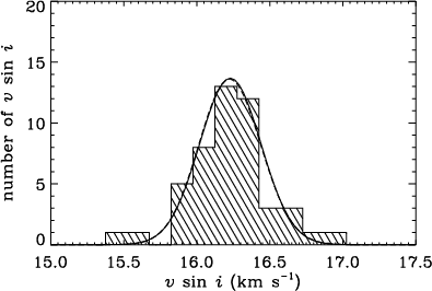
Distribution of observational errors, in the case of rotational velocities, is of particular interest during a deconvolution process in order to get rid of statistical errors in a significant sample.
To have an idea of the shape of the error law associated with the
![]() ,
it is necessary to have a great number of spectra for the same star.
Sirius has been observed on several occasions during the runs and its spectrum has been collected 48 times. Sirius spectra typically exhibit high signal-to-noise ratio (
,
it is necessary to have a great number of spectra for the same star.
Sirius has been observed on several occasions during the runs and its spectrum has been collected 48 times. Sirius spectra typically exhibit high signal-to-noise ratio (
![]() ). The 48 values derived from each set of lines, displayed in Fig. 11, give us an insight into the errors distribution. The mean
). The 48 values derived from each set of lines, displayed in Fig. 11, give us an insight into the errors distribution. The mean
![]() is
is
![]()
![]() and its associated standard deviation
and its associated standard deviation
![]()
![]() ;
data are approximatively distributed following a Gaussian around the mean
;
data are approximatively distributed following a Gaussian around the mean
![]() .
.
Moreover, for higher broadening, the impact of the sampling effect of
the FT (Eq. (6)) is foreseen, resulting in a distribution with a box-shaped profile. This effect becomes noticeable for
![]()
![]() .
.
Copyright ESO 2001

![\begin{table}
\includegraphics[width=12cm,clip]{test1.ps}\end{table}](/articles/aa/full/2002/01/aa1414/imgbis.gif)