The intensities of the three lines (resonance, forbidden and intercombination) are calculated mainly from atomic data presented in Paper I (Porquet & Dubau 2000). In this work (as well as in Paper I) for all temperatures (low and high), radiative recombination contributions (direct + upper-level radiative cascades), and collisional excitations inside the n=2 shell were included in the line ratio calculations. For high temperatures, the collisional excitation contribution (direct + near-threshold resonance + cascades) from the ground level (n=1 shell, 1s2) are important as well as dielectronic recombination (direct + cascades).
Excitation collisional data are also taken from Paper I, which are based on the calculations from Zhang & Sampson (1987) plus the contribution of the upper-level (n>2) radiative cascades calculated in Paper I (see Paper I for more details).
The ionization balance is from Mazzotta et al. (1998) and the data for radiative and dielectronic recombinations are from Paper I. Various new data for the transition probabilities (e.g., forbidden and intercombination lines) have been selected (see Sect. 4.1).
In the following paragraphs we describe the several differences between Paper I and this work: Aki, optical depth, contribution of the blended dielectronic satellite lines, and radiation field.
| ion | forbidden line | intercombination line |
| (z, |
(y, |
|
| C V | 4.857(+1) (S94) | 2.90(+7) (H85) |
| N VI | 2.538(+2) (N00) | 1.38(+8) (H85) |
| O VII | 1.046(+3) (C98) | 5.800(+8) (E81) |
| Ne IX | 1.09(+4) (T99) | 5.400(+9) * |
| Mg XI | 7.347(+4) (S95) | 3.448(+10) (A81) |
| Si XIII | 3.610(+5) * | 1.497(+11) (A79) |
(A79): Armour et al. (1979)
(A81): Armour et al. (1981)
(C98): Crespo López-Urrutia et al. (1998)
(E81): Engström et al. (1981)
(H85): Hutton et al. (1985)
(N00): Neill et al. (2000)
(S94): Schmidt et al. (1994)
(S95): Stefanelli et al. (1995)
(T99): Träbert et al. (1999)
*: Theoretical values taken from Lin et al. (1977), see text (Sect. 4.1).
We have updated the transition probabilities Aki reported in Paper I
for the intercombination (y, ![]() )
and the forbidden (z,
)
and the forbidden (z, ![]() )
line by published experimental values (see Table 2, and references therein). In some cases, no published
experimental values have been found and then we used the theoretical values from Lin et al. (1977).
Indeed, comparisons of their theoretical values with the experimental values reported in
Table 2 seem to show good agreement in other cases.
)
line by published experimental values (see Table 2, and references therein). In some cases, no published
experimental values have been found and then we used the theoretical values from Lin et al. (1977).
Indeed, comparisons of their theoretical values with the experimental values reported in
Table 2 seem to show good agreement in other cases.
For C V, the ratio R is reduced by about 20![]() comparing the calculations using the values of
Aki reported in Paper I, while for N VI the reduction is
less than
comparing the calculations using the values of
Aki reported in Paper I, while for N VI the reduction is
less than ![]() .
For O VII, Ne IX, Mg XI, and Si XIII, the differences
between the current calculations using these new values of Aki and those reported in Paper I are negligible.
.
For O VII, Ne IX, Mg XI, and Si XIII, the differences
between the current calculations using these new values of Aki and those reported in Paper I are negligible.
Schrijver et al. (1995) and Mewe et al. (1995b) have investigated the possibility that
resonance photons are scattered out of the line of sight in late-type stellar coronae (see also Acton 1978).
Indeed, in this process, a resonance line photon is absorbed by an ion in the ground state and then re-emitted,
generally in a different direction. So, the total photon intensity integrated over 4![]() remains unchanged
but the photon distribution with respect to a given direction is altered. This absorption and re-emission is
indistinguishable from scattering and depends on the geometry of the region being observed. In general,
photons would be scattered preferentially out of the line of sight for active regions (relatively dense areas)
and into the line of sight for the surrounding quiet Sun (less dense area), see Schmelz et al.
(1997) and Mewe et al. (2001). The effect is smaller for instruments with a
larger field of view.
remains unchanged
but the photon distribution with respect to a given direction is altered. This absorption and re-emission is
indistinguishable from scattering and depends on the geometry of the region being observed. In general,
photons would be scattered preferentially out of the line of sight for active regions (relatively dense areas)
and into the line of sight for the surrounding quiet Sun (less dense area), see Schmelz et al.
(1997) and Mewe et al. (2001). The effect is smaller for instruments with a
larger field of view.
This could have an impact on the temperature diagnostic, the so-called G=(z+x+y)/w or (f+i)/r ratio. If the optical depth of the line is not taken into account, the calculated intensity ratio G can be overestimated and the inferred temperature from the G ratio is underestimated.
As detailed in Mewe et al. (2001), branching ratios can be used to check the assumption of the
optical thin model because effects of resonance scattering would affect the measured branching ratio. From
the fact that the intensities of e.g., the strong resonance lines Fe XVIII![]() 93.92 and
Fe XIX
93.92 and
Fe XIX![]() 108.307 are in good agreement with the intensities of other lines sharing the same
upper level, one can derive a constraint on the optical depth taking into account the systematic
uncertainties of the theoretical transition probabilities A (typical 25
108.307 are in good agreement with the intensities of other lines sharing the same
upper level, one can derive a constraint on the optical depth taking into account the systematic
uncertainties of the theoretical transition probabilities A (typical 25![]() for each A, hence 35
for each A, hence 35![]() for
the branching ratio) which dominate over the statistical errors (typically 10
for
the branching ratio) which dominate over the statistical errors (typically 10![]() ). If we rule out a
reduction in the resonance line intensity larger than about 30
). If we rule out a
reduction in the resonance line intensity larger than about 30![]() ,
then on the basis of a simple
"escape-factor'' model with
,
then on the basis of a simple
"escape-factor'' model with
 |
(24) |
 |
(25) |
Since
![]() (
(
![]() and
and
![]() corresponding respectively to the optical depth of
the resonance and the intercombination lines), we can write
corresponding respectively to the optical depth of
the resonance and the intercombination lines), we can write
![]() ,
where
,
where ![]() is the value of the ratio taken into account the optical depth of the resonance line,
G is the value without resonant scattering (such as in Paper I and Sect. 5), and
is the value of the ratio taken into account the optical depth of the resonance line,
G is the value without resonant scattering (such as in Paper I and Sect. 5), and
![]() is the escape probability for the resonance line (Eq. (22)).
One should note that
is the escape probability for the resonance line (Eq. (22)).
One should note that ![]() is not strictly exact when the contribution of the blended dielectronic satellite lines are
introduced in the calculations (see Sect. 4.3).
is not strictly exact when the contribution of the blended dielectronic satellite lines are
introduced in the calculations (see Sect. 4.3).
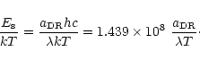
The intensity of a dielectronic satellite line arising from a doubly excited state with principal quantum number n
in a Lithium-like ion produced by dielectronic recombination of a He-like ion is given by:
| (26) |
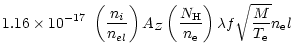
The rate coefficient (in cm3s-1) for dielectronic recombination is given by (Bely-Dubau et al. 1979):
 |
(27) |
 |
(28) |
For a group of satellites with the same principal quantum
number n, ![]() can be approximated by
can be approximated by
 |
(30) |
For the n=2, 3, 4 blended dielectronic satellite lines we use the atomic data reported in the Appendix.
For the higher-n blended dielectronic satellite lines we use the results from Karim and co-workers.
For Z=10 (Ne IX) we use the data from Karim (1993) who gives the intensity factor
![]() for
the strongest (
F*2 > 1012s-1) dielectronic satellite lines with n=5-8. For Z=14 (Si XIII),
we take the calculations from Karim & Bhalla (1992) who report the intensity factor
F*2 for the strongest (
F*2 > 1012s-1) dielectronic satellite lines
with n=5-8. For Z=12 (Mg XI) we have interpolated between the calculations from Karim (1993) for
Z=10, and from
Karim & Bhalla (1992) for Z=14.
for
the strongest (
F*2 > 1012s-1) dielectronic satellite lines with n=5-8. For Z=14 (Si XIII),
we take the calculations from Karim & Bhalla (1992) who report the intensity factor
F*2 for the strongest (
F*2 > 1012s-1) dielectronic satellite lines
with n=5-8. For Z=12 (Mg XI) we have interpolated between the calculations from Karim (1993) for
Z=10, and from
Karim & Bhalla (1992) for Z=14.
Including the contribution of the blended dielectronic satellite lines, we write for the ratios R and G:
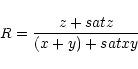 |
(31) |
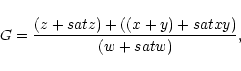 |
(32) |
At the temperature at which the ion fraction is maximum for the He-like ion
(see e.g. Arnaud & Rothenflug 1985; Mazzotta et al. 1998), the differences between the
calculations for R (for G) with or without taking into account the blended dielectronic satellite lines are only
of about 1![]() (9
(9![]() ),
), ![]() (5
(5![]() ), and 5
), and 5![]() (3
(3![]() )
for Ne IX, Mg XI, and
Si XIII at the low-density limit and for
)
for Ne IX, Mg XI, and
Si XIII at the low-density limit and for
![]() K, respectively. On the other hand, for much
lower electron temperatures, the effect is bigger since the intensity of
the dielectronic satellite lines is proportional to
K, respectively. On the other hand, for much
lower electron temperatures, the effect is bigger since the intensity of
the dielectronic satellite lines is proportional to
![]() .
As well, for high values of density
(
.
As well, for high values of density
(![]() )
at which the intensity of the forbidden line is very weak (i.e. tends to zero), the
contribution of the blended dielectronic satellite lines to the forbidden line leads to a ratio R which decreases much
slower with
)
at which the intensity of the forbidden line is very weak (i.e. tends to zero), the
contribution of the blended dielectronic satellite lines to the forbidden line leads to a ratio R which decreases much
slower with ![]() than in the case where the contribution of the blended dielectronic satellite lines is not taken
into account.
than in the case where the contribution of the blended dielectronic satellite lines is not taken
into account.
Recently, Kahn et al. (2001) have found with the RGS on XMM-Newton
that for ![]() Puppis, the forbidden to
intercombination line ratios within the helium-like triplets are abnormally low for N VI,
O VII, and Ne IX. While this is sometimes indicative of a high electron density,
they have shown that
in the case of
Puppis, the forbidden to
intercombination line ratios within the helium-like triplets are abnormally low for N VI,
O VII, and Ne IX. While this is sometimes indicative of a high electron density,
they have shown that
in the case of ![]() Puppis, it is instead caused by the intense radiation field of this star. This constrains
the location of the X-ray emitting shocks relative to the star, since the emitting regions should be close enough
to the star in order that the UV radiation is not diluted too much.
A strong radiation field can mimic a high density if the upper (3S) level of the forbidden line
is significantly depopulated via photo-excitation to the upper (3P) levels
of the intercombination lines,
analogously to the effect of electronic collisional excitation (Fig. 1).
The result is an increase of the intercombination
lines and a decrease of the forbidden line.
Puppis, it is instead caused by the intense radiation field of this star. This constrains
the location of the X-ray emitting shocks relative to the star, since the emitting regions should be close enough
to the star in order that the UV radiation is not diluted too much.
A strong radiation field can mimic a high density if the upper (3S) level of the forbidden line
is significantly depopulated via photo-excitation to the upper (3P) levels
of the intercombination lines,
analogously to the effect of electronic collisional excitation (Fig. 1).
The result is an increase of the intercombination
lines and a decrease of the forbidden line.
Equation (21) gives the expression for photo-excitation from level m to level pk in a radiation field
with effective blackbody temperature
![]() from a hot star underlying the X-ray line emitting plasma. As pointed
out by Mewe & Schrijver (1978a) the radiation is diluted by a factor W given by
from a hot star underlying the X-ray line emitting plasma. As pointed
out by Mewe & Schrijver (1978a) the radiation is diluted by a factor W given by
![\begin{displaymath}%
W=\frac{1}{2}~\left[1-\left(1-\left(\frac{r_{*}}{r}\right)\right)^{1/2}\right],
\end{displaymath}](/articles/aa/full/2001/36/aa1442/img123.gif) |
(33) |
In their Table 8, Mewe & Schrijver (1978a) give for information the radiation temperature for a
solar photospheric field for Z=6, 7, and 8. In Table 3, we report the wavelengths at
which the radiation temperature should be estimated for Z=6, 7, 8, 10, 12, 14.
These wavelengths correspond to the transitions between the 3S and 3P levels (
![]() )
and the
1S and 1P levels (
)
and the
1S and 1P levels (
![]() ).
).
| C V | N VI | O VII | Ne IX | Mg XI | Si XIII | |
|
|
2280 | 1906 | 1637 | 1270 | 1033 | 864 |
|
|
3542 | 2904 | 2454 | 1860 | 1475 | 1200 |
The photo-excitation from the 3S level and 3P levels is very important for low-Z ions C V,
N VI, O VII. For higher-Z ions, this process is only important for very high radiation temperature
(![]() few 10000 K).
few 10000 K).
One can note that the photo-excitation between the levels 1S0 and 1P1 is negligible compared
to the photo-excitation between the 3S1 and 3P0,1,2 levels. For example, for a very high
value of
![]() K the difference between the calculations taken or not taken into account the
photo-excitation between 1S0 and 1P1 is smaller than 20
K the difference between the calculations taken or not taken into account the
photo-excitation between 1S0 and 1P1 is smaller than 20![]() for C V, where this effect
is expected to be maximum.
for C V, where this effect
is expected to be maximum.
Copyright ESO 2001
![\begin{displaymath}
%
P(\tau) \simeq \frac{1}{[1+0.43 \tau]},
\end{displaymath}](/articles/aa/full/2001/36/aa1442/img76.gif)
![\begin{displaymath}
%
E_{\rm s} [\rm eV] = 1.239842\times 10^4 \ {a_{DR}\over {\lambda}},
\end{displaymath}](/articles/aa/full/2001/36/aa1442/img110.gif)