The present numerical code is modified from our previously published Monte Carlo code (Vainio et al. 2000). Similar transport codes, including also non-linear effects, have been developed previously (e.g., Ellison et al. 1996), but to our knowledge, ours is the first Monte Carlo code to employ self-generated waves.
When the Monte Carlo particles (numbered by j) are injected in the simulation,
they are a given a weight wj that normalizes their injection rate to the
physical value given by Q. The particles are treated in the guiding center
approximation, which in the present case of constant magnetic field strength
means that during the Monte Carlo time step, ![]() ,
we move the particles in
the spatial coordinate (measured along the field lines) as
,
we move the particles in
the spatial coordinate (measured along the field lines) as
![]() ,
where vj and
,
where vj and ![]() are the particle
speed and pitch-angle cosine of the jth particle as measured in the fixed
frame, where the background plasma is assumed to be stationary. In addition, the
particles suffer scatterings from two Alfvén wave fields propagating parallel
and anti-parallel to the magnetic field. In scatterings, performed after each
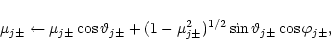
Monte Carlo time step modeling pitch-angle diffusion, the particles are
subsequently scattered (elastically) in the two wave frames, first
Lorentz-transforming the particle velocity to the wave frame, then using
are the particle
speed and pitch-angle cosine of the jth particle as measured in the fixed
frame, where the background plasma is assumed to be stationary. In addition, the
particles suffer scatterings from two Alfvén wave fields propagating parallel
and anti-parallel to the magnetic field. In scatterings, performed after each
Monte Carlo time step modeling pitch-angle diffusion, the particles are
subsequently scattered (elastically) in the two wave frames, first
Lorentz-transforming the particle velocity to the wave frame, then using
 |
(A.1) |
We keep track of the wave energy densities on a spatial grid with N=150elements numbered by i=1,...,N, and with a spacing of
![]() and
central coordinates x=Xi. The value of
and
central coordinates x=Xi. The value of
![]() is taken to be
constant inside each grid cell. Thus,
is taken to be
constant inside each grid cell. Thus,
![]() and
ij is the index of the grid cell that contains xj, i.e.,
and
ij is the index of the grid cell that contains xj, i.e.,
![]() ,
where
,
where
![]() .
During each
Monte Carlo time step, a change of the wave energy density due to wave-particle
interactions is computed from
.
During each
Monte Carlo time step, a change of the wave energy density due to wave-particle
interactions is computed from
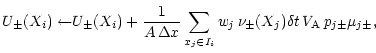 | (A.2) | ||
In addition to the wave-particle interactions, the waves are convected on the
grid by
![]() if
if
![]() and
U+[-](X1[N])=U0, each time the simulation time t has
elapsed an amount of
and
U+[-](X1[N])=U0, each time the simulation time t has
elapsed an amount of
![]() .
At boundaries, the wave energy
convected out of the grid is lost.
.
At boundaries, the wave energy
convected out of the grid is lost.
As an output, the simulation code saves the momentum, pitch-angle cosine and
escape time of all particles leaving the simulation box. In addition, the
wave-energy densities and the energetic particle pressure inside the simulation
box is saved after every time the waves are moved on the grid, i.e., at
t mod
![]() .
To illustrate the typical development of a
simulation, we have plotted in Fig. A.1 the wave-energy densities
and particle pressures in a few frames for simulation in Case B with source
position at
.
To illustrate the typical development of a
simulation, we have plotted in Fig. A.1 the wave-energy densities
and particle pressures in a few frames for simulation in Case B with source
position at ![]() (see Fig. 3 for the escaping particle
flux).
(see Fig. 3 for the escaping particle
flux).
As an outline of the future work, we note that a generalization to a spectrum of
Alfvén waves would mean that the wave-energy density grid would contain another
dimension (wavenumber), and that the resonance condition would have to be taken
into account in deciding which particles contribute the the growth of the waves
in the particular grid element. If one uses the full quasi-linear resonance
condition with ![]() -dependence, one has to also take this into account when
modeling the scattering frequency, which has to be allowed a
-dependence, one has to also take this into account when
modeling the scattering frequency, which has to be allowed a ![]() -dependence.
This, naturally, affects also the growth rate of the waves. The effects of
non-constant magnetic field to the particle transport are easy to take into
account (Vainio et al. 2000); for wave transport, one has to use an
equation that employs the diverging field effects as well as the effects of a
non-constant group speed.
-dependence.
This, naturally, affects also the growth rate of the waves. The effects of
non-constant magnetic field to the particle transport are easy to take into
account (Vainio et al. 2000); for wave transport, one has to use an
equation that employs the diverging field effects as well as the effects of a
non-constant group speed.
Copyright ESO 2001
![\begin{figure}
\includegraphics[width=16.1cm,clip]{ms1322fn.eps}
\end{figure}](/articles/aa/full/2001/31/aa1322/img137.gif)