In the first set of simulations, we study a loop which is spatially symmetric
about the point source of energetic protons. We inject
![]() (corresponding to an energy of about 30 MeV) protons isotropically at a rate
(corresponding to an energy of about 30 MeV) protons isotropically at a rate
![]() cm-2 s-1,
where
cm-2 s-1,
where
![]() is chosen to give a large flux resulting in a
rapid wave growth, but still keeping the energetic-proton pressure at least an
order of magnitude below the thermal proton pressure even if all particles are
trapped by Alfvén waves inside
is chosen to give a large flux resulting in a
rapid wave growth, but still keeping the energetic-proton pressure at least an
order of magnitude below the thermal proton pressure even if all particles are
trapped by Alfvén waves inside
![]() .
We vary the total amount of
injected particles by varying the duration of the injection between
.
We vary the total amount of
injected particles by varying the duration of the injection between
![]() s and 10/15 s, resulting in a total number of injected particles
between
s and 10/15 s, resulting in a total number of injected particles
between
![]() cm-2 and
cm-2 and
![]() cm-2. The background wave flux emitted from the footpoints is fixed by
assuming that the wave mode emitted from each footpoint has an energy density of
cm-2. The background wave flux emitted from the footpoints is fixed by
assuming that the wave mode emitted from each footpoint has an energy density of
![]() .
We assume that this emission
of waves is steady; thus the initial condition for both wave modes is also
.
We assume that this emission
of waves is steady; thus the initial condition for both wave modes is also
![]() .
The adopted value for 2U0 corresponds to an rms
velocity amplitude of 10 kms-1 per logarithmic bandwidth at
.
The adopted value for 2U0 corresponds to an rms
velocity amplitude of 10 kms-1 per logarithmic bandwidth at
![]() kHz. Assuming that this velocity amplitude
holds for all frequencies from
f0=VA/L=0.1 Hz up to
kHz. Assuming that this velocity amplitude
holds for all frequencies from
f0=VA/L=0.1 Hz up to
![]() kHz, the total rms
amplitude is 38 kms-1, which agrees very well with the typical observed
non-thermal velocity in a quiescent active region of 45 km s-1 (Antonucci
& Dodero 1995). The non-thermal velocities in flaring plasmas are
larger, consistent with wave growth. We do not consider any emission of waves
from the acceleration site; we assume that the waves are absorbed by the
particles during the acceleration. However, some external forcing of the
Alfvénic turbulence is modeled by keeping the wave-energy densities above a
minimum level of
kHz, the total rms
amplitude is 38 kms-1, which agrees very well with the typical observed
non-thermal velocity in a quiescent active region of 45 km s-1 (Antonucci
& Dodero 1995). The non-thermal velocities in flaring plasmas are
larger, consistent with wave growth. We do not consider any emission of waves
from the acceleration site; we assume that the waves are absorbed by the
particles during the acceleration. However, some external forcing of the
Alfvénic turbulence is modeled by keeping the wave-energy densities above a
minimum level of
![]() everywhere
inside the flux tube.
everywhere
inside the flux tube.
The results of the simulations are presented in Fig. 1
in form of flux of protons precipitating at the footpoints of the loop. One can
see a peak in the precipitating flux at
![]() s corresponding to the
travel time of Alfvén waves from the center of the loop to the footpoints, as
predicted by the theory of Bespalov et al. (1987, 1991). What
is not predicted by the steady-state theory is the rather intense precursor peak
immediately after the particle release, that corresponds to the first phase,
when the waves have not yet grown enough to suppress the diffusive particle
transport. The number of particles in the precursor seems to be independent of
the number of injected particles, if this number exceeds a threshold level.
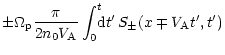
This can be understood as follows. We consider an initial turbulence level,
where the diffusion length,
s corresponding to the
travel time of Alfvén waves from the center of the loop to the footpoints, as
predicted by the theory of Bespalov et al. (1987, 1991). What
is not predicted by the steady-state theory is the rather intense precursor peak
immediately after the particle release, that corresponds to the first phase,
when the waves have not yet grown enough to suppress the diffusive particle
transport. The number of particles in the precursor seems to be independent of
the number of injected particles, if this number exceeds a threshold level.
This can be understood as follows. We consider an initial turbulence level,
where the diffusion length,
![]() (where
(where
![]() is the spatial diffusion coefficient), is larger than the
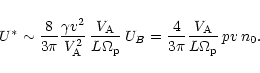
distance from the source to the footpoints. Until the wave-energy density has
grown to a level, denoted by U*, that suppresses diffusive transport, the
particles propagate quickly (relative to the time scale of wave transport)
towards the footpoints adjusting the value of particle flux to
is the spatial diffusion coefficient), is larger than the
distance from the source to the footpoints. Until the wave-energy density has
grown to a level, denoted by U*, that suppresses diffusive transport, the
particles propagate quickly (relative to the time scale of wave transport)
towards the footpoints adjusting the value of particle flux to
![]() (directed away from the source). The wave-energy density
obeys
(directed away from the source). The wave-energy density
obeys
 |
= | 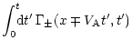 |
|
| = |  |
||
| (3) |
 |
(5) |
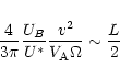
Let us estimate the spectrum of the promptly-precipitating protons. If a
spectrum of particles is emitted, and if energy changes during the transport are
neglected, we should identify the number of precursor protons with
![]() in the spirit of the
resonance condition
in the spirit of the
resonance condition
![]() .
For a wave spectrum
.
For a wave spectrum
![]() with q<3,
with q<3,
![]() increases with (non-relativistic) energy, although
logarithmically (
increases with (non-relativistic) energy, although
logarithmically (
![]() ). Typical turbulence models give
1<q<2. Up to the energy where the total number of injected particles (per
logarithmic momentum interval),
). Typical turbulence models give
1<q<2. Up to the energy where the total number of injected particles (per
logarithmic momentum interval),
![]() ,
equals the calculated value for the precursor,
Eqs. (4-6), the energy spectrum of the first peak is
,
equals the calculated value for the precursor,
Eqs. (4-6), the energy spectrum of the first peak is
![]() .
At larger energies, only the first peak is observed with a
spectrum identical to that of the source.
.
At larger energies, only the first peak is observed with a
spectrum identical to that of the source.
Using the assumption of a steady state, Bespalov et al. (1991) deduced
that the rate of particle injection determines whether particle transport is
governed by diffusion or convection with the waves. That is correct in the
steady-state regime of continual injection. In the case of short injection,
however, the total number of injected particles, ![]() ,
is the only
controlling factor in the relative importance of the prompt and delayed
components of the precipitating flux. To confirm this, we ran a simulations of
using injection rates of
,
is the only
controlling factor in the relative importance of the prompt and delayed
components of the precipitating flux. To confirm this, we ran a simulations of
using injection rates of
![]() ,
,
![]() ,
and
,
and
![]() and with
and with
![]() cm-2 in all cases
(Fig. 2). The resulting flux of precipitating particles
looks nearly identical for the shortest injections (
cm-2 in all cases
(Fig. 2). The resulting flux of precipitating particles
looks nearly identical for the shortest injections (
![]() s and 1/3 s) since the diffusive time scale is large enough to regard both of these
injections as impulsive. The prolonged injection (
s and 1/3 s) since the diffusive time scale is large enough to regard both of these
injections as impulsive. The prolonged injection (
![]() s), however,
suppresses the height of the precursor while keeping the total number of
precursor particles very similar to the impulsive ones, which is in accord with
diffusive transport. Further, increasing the loop length or the level of ambient
turbulence inside the loop clearly suppresses the importance of the precursor
predicted by the estimation and confirmed by simulations. We, thus, regard the
Eqs. (4-6), up to a numerical factor of the order unity,
as a valid scaling law for arranging observations of precipitating proton
fluences.
s), however,
suppresses the height of the precursor while keeping the total number of
precursor particles very similar to the impulsive ones, which is in accord with
diffusive transport. Further, increasing the loop length or the level of ambient
turbulence inside the loop clearly suppresses the importance of the precursor
predicted by the estimation and confirmed by simulations. We, thus, regard the
Eqs. (4-6), up to a numerical factor of the order unity,
as a valid scaling law for arranging observations of precipitating proton
fluences.
![\begin{figure}
\includegraphics[width=8.7cm,clip]{ms1322f2.eps}
\end{figure}](/articles/aa/full/2001/31/aa1322/img85.gif) |
Figure 2:
Precipitating flux for a constant number of injected particles,
|
As became evident from the simulations of Case A, the majority of the particles
in a powerful impulsive flare precipitate once the turbulent walls have reached
the footpoints of the flux tube, at
t=L/2VA. It is of interest to
investigate what happens if the particles are not released in the central point
of the flux tube; if the trap reaches one end first, we should see a peak in the
precipitating flux at this footpoint, but if the precipitation is rapid, the
particle reservoir might empty before the trap opens from the other end. We
have simulated this by varying the position of the source as
![]() ,
,
![]() ,
and
,
and ![]() (from the center of the loop). The number of injected
particles was
(from the center of the loop). The number of injected
particles was
![]() cm-2, and other parameters were chosen
as in Case A. The results are plotted in Fig. 3. The flux
towards the footpoint closer to the source resembles the symmetric case with a
prompt and a delayed peak. The flux at the other footpoint, however, behaves
differently. Even a slightly asymmetric position of the source can lead to a
huge difference in the precipitating flux for the delayed component; in
practice, we can expect a delayed brightening in
cm-2, and other parameters were chosen
as in Case A. The results are plotted in Fig. 3. The flux
towards the footpoint closer to the source resembles the symmetric case with a
prompt and a delayed peak. The flux at the other footpoint, however, behaves
differently. Even a slightly asymmetric position of the source can lead to a
huge difference in the precipitating flux for the delayed component; in
practice, we can expect a delayed brightening in ![]() -rays at only one of
the footpoints based on our simulations. However, the observed asymmetry in the
precursor brightening provides a measure of the asymmetry of the source
position, if the ambient turbulence level is high enough to yield a diffusive
delay in the particle flux reaching the footpoints at different distances from
the source.
-rays at only one of
the footpoints based on our simulations. However, the observed asymmetry in the
precursor brightening provides a measure of the asymmetry of the source
position, if the ambient turbulence level is high enough to yield a diffusive
delay in the particle flux reaching the footpoints at different distances from
the source.
Without a possibility to distinguish between the emission from different footpoints, the observations in the asymmetric case are very similar to the symmetric case, and the general conclusions drawn from Case A - two-component structure, importance of the total number of injected particles - are valid also for the asymmetric case.
As a last study, we performed simulations in a flux tube that is connected to
the solar surface from one footpoint at x=0, only. The other end at
![]() cm is assumed to leak the incident particles directly to
the interplanetary medium, modeling a flux tube rapidly expanding above x=L;
a large and rapid expansion would probably eject most of the particles reaching
this distance, since the particle bulk speed is directed outwards, and particles
diffusing backward relative to the flow at
cm is assumed to leak the incident particles directly to
the interplanetary medium, modeling a flux tube rapidly expanding above x=L;
a large and rapid expansion would probably eject most of the particles reaching
this distance, since the particle bulk speed is directed outwards, and particles
diffusing backward relative to the flow at
![]() see the boundary as a
strong magnetic mirror. In a more gently opening geometry, the effects of the
diverging field should be taken into account explicitly in the simulation. The
source is positioned at
see the boundary as a
strong magnetic mirror. In a more gently opening geometry, the effects of the
diverging field should be taken into account explicitly in the simulation. The
source is positioned at ![]() ,
and the total number of injected particles
is
,
and the total number of injected particles
is
![]() cm-2. This case differs from Case B simulations
in that we assume that the background Alfvén waves have a large cross helicity:
the outward propagating waves have
cm-2. This case differs from Case B simulations
in that we assume that the background Alfvén waves have a large cross helicity:
the outward propagating waves have
![]() as in Cases A and B, but
the inward propagating waves have only the minimum-level intensity,
as in Cases A and B, but
the inward propagating waves have only the minimum-level intensity,
![]() .
Other parameters were taken as in
Cases A and B.
.
Other parameters were taken as in
Cases A and B.
The results of the open-field simulation are shown in Fig. 4. The precipitating particle flux again shows a double peaked structure, with a precursor well described by Eqs. (4-6). The escaping flux, however, rises more slowly to a stationary level that is destroyed by the boundary effects, when the turbulent trap hits the free-escape boundary, opening it also from this end. Towards the end of the event, the escaping flux becomes dominant over the precipitating flux. The number of precipitating particles is, however, an order of magnitude larger than the number of escaping particles, which shows that energetic particles accelerated in impulsive flares can be effectively trapped near the Sun even on open field lines. This demonstrates that the small ratio of interplanetary-to-interacting protons observed in impulsive flares do not necessarily result from closed field line topology.
Copyright ESO 2001
![\begin{figure}
\includegraphics[width=8.2cm,clip]{ms1322f1.eps}
\end{figure}](/articles/aa/full/2001/31/aa1322/img68.gif)
![\begin{figure}
\includegraphics[width=8.2cm,clip]{ms1322f3.eps}
\end{figure}](/articles/aa/full/2001/31/aa1322/img86.gif)
![\begin{figure}
\includegraphics[width=8.27cm,clip]{ms1322f4.eps}
\end{figure}](/articles/aa/full/2001/31/aa1322/img92.gif)