As noted elsewhere (e.g. Bernardeau et al. 1997; Jain & Seljak 1997), the parameters which
dominate the 2-point shear statistics are the power
spectrum normalization ![]() and the mean density
and the mean density ![]() .
We investigate below how the statistics measured
in Figs. 3 to 6 are consistent with each other
when constraining these
parameters. Our parameter estimates below rely on some simplifying
assumptions; a more detailed analysis over a wider space of parameters
will be presented elsewhere. In particular, as discussed later, the choice of
the slope of the power spectrum
.
We investigate below how the statistics measured
in Figs. 3 to 6 are consistent with each other
when constraining these
parameters. Our parameter estimates below rely on some simplifying
assumptions; a more detailed analysis over a wider space of parameters
will be presented elsewhere. In particular, as discussed later, the choice of
the slope of the power spectrum ![]() is weakly known, and may significantly affect
the parameter estimate. As pointed out in Sect. 4,
the uncertainty on the redshift distribution is also a
concern, but we partialy address this point by constraining the parameters using three
different redshift distributions. A complete analysis involving marginalisation
over
is weakly known, and may significantly affect
the parameter estimate. As pointed out in Sect. 4,
the uncertainty on the redshift distribution is also a
concern, but we partialy address this point by constraining the parameters using three
different redshift distributions. A complete analysis involving marginalisation
over ![]() and the redshift distribution using tight priors is left for a
future work.
and the redshift distribution using tight priors is left for a
future work.
We assume that the data follow Gaussian statistics and neglect sample variance
since it is a very small contributor to the noise for
our survey, as discussed above. We compute the likelihood function ![]() :
:
Figure 4 (bottom panel) shows that for effective scales
smaller than 1' there is a non-vanishing R-mode which could come either
from a residual systematic, or from an intrinsic alignment effect. Therefore
it is safer to exclude this part from the likelihood calculation:
for the top-hat variance, we excluded the point at 1', for the correlation
functions the points below 2', and for the
![]() statistic the points
below 5'. For the correlation function, we also excluded the points at
scales larger than 20' because of the small fluctuations in the measured
correlations. The constraints
on the cosmological parameters are not significantly affected whether
these large scale points are excluded or not.
statistic the points
below 5'. For the correlation function, we also excluded the points at
scales larger than 20' because of the small fluctuations in the measured
correlations. The constraints
on the cosmological parameters are not significantly affected whether
these large scale points are excluded or not.
![\begin{figure}
\par\includegraphics[width=6.6cm,clip]{new_omega_sigma_var.ps}
\end{figure}](/articles/aa/full/2001/30/aa1091/img131.gif) |
Figure 9:
Likelihood contours
in the
|
Figures 9 to 13 show the
![]() constraints for each of the statistics shown in
Figs. 3 to 6. The contours show the
constraints for each of the statistics shown in
Figs. 3 to 6. The contours show the ![]() ,
,
![]() and
and ![]() confidence levels. The agreement between the
contours is excellent, though the
confidence levels. The agreement between the
contours is excellent, though the
![]() statistic and the radial
correlation function do not give as tight constraints as the other
statistics. The correlation function measurements below
2' may be considered by using error bars that include a possible
systematic bias: this is equivalent to adding a systematic
covariance matrix
statistic and the radial
correlation function do not give as tight constraints as the other
statistics. The correlation function measurements below
2' may be considered by using error bars that include a possible
systematic bias: this is equivalent to adding a systematic
covariance matrix
![]() to the noise covariance
to the noise covariance ![]() matrix
in Eq. (18). The new contours
computed with the enlarged error
bars
matrix
in Eq. (18). The new contours
computed with the enlarged error
bars![]() are shown
in Fig. 14.
The maximum of the likelihood in the variance and correlation function
likelihood plots is at
are shown
in Fig. 14.
The maximum of the likelihood in the variance and correlation function
likelihood plots is at
![]() and
and
![]() .
Note that the results are in very good agreement
.
Note that the results are in very good agreement![]() with a similar plot in Maoli et al. (2001)
(Fig. 8), here the contours are narrower, and are obtained
from a homogeneous data set. Moreover, the degeneracy
between
with a similar plot in Maoli et al. (2001)
(Fig. 8), here the contours are narrower, and are obtained
from a homogeneous data set. Moreover, the degeneracy
between ![]() and
and ![]() is broken.
is broken.
![\begin{figure}
\par\includegraphics[width=6.4cm,clip]{new_omega_sigma_map.ps}
\end{figure}](/articles/aa/full/2001/30/aa1091/img139.gif) |
Figure 10:
As in Fig. 9,
but using the
|
![\begin{figure}
\par\includegraphics[width=6.4cm,clip]{new_omega_sigma_gg.ps}
\end{figure}](/articles/aa/full/2001/30/aa1091/img140.gif) |
Figure 11:
Likelihood contours
as in Fig. 9,
but using the shear correlation function
|
![\begin{figure}
\par\includegraphics[width=6.4cm,clip]{new_omega_sigma_etet.ps}
\end{figure}](/articles/aa/full/2001/30/aa1091/img141.gif) |
Figure 12:
As in Fig. 9,
but using the tangential shear correlation function
|
![\begin{figure}
\par\includegraphics[width=6.4cm,clip]{new_omega_sigma_erer.ps}
\end{figure}](/articles/aa/full/2001/30/aa1091/img142.gif) |
Figure 13:
As in Fig. 9,
but using the radial shear correlation function
|
The partial breaking of degeneracy between
![]() and
and ![]() was expected from the fully non-linear calculation of shear correlations
(Jain & Seljak 1997). In the non-linear regime the dependence of the
2-points statistics on
was expected from the fully non-linear calculation of shear correlations
(Jain & Seljak 1997). In the non-linear regime the dependence of the
2-points statistics on ![]() and
and ![]() becomes
sensitive to angular scale.
For example, as shown in Jain & Seljak (1997),
the shear rms measures
becomes
sensitive to angular scale.
For example, as shown in Jain & Seljak (1997),
the shear rms measures
![]() on scale between 2'-5',
and
on scale between 2'-5',
and
![]() on scales
on scales
![]() .
Therefore a low
.
Therefore a low ![]() universe should see a net decrease of shear power at large scale compared to
a
universe should see a net decrease of shear power at large scale compared to
a
![]() universe (for a given shape of the power spectrum),
as is evident in Fig. 3. Note that the aperture mass
universe (for a given shape of the power spectrum),
as is evident in Fig. 3. Note that the aperture mass
![]() is still degenerate with
is still degenerate with ![]() and
and ![]() (Fig. 10) because it probes effective scales up to
(Fig. 10) because it probes effective scales up to
![]() only, which is not enough to break the degeneracy.
only, which is not enough to break the degeneracy.
![\begin{figure}
\par\includegraphics[width=6.4cm,clip]{new_omega_sigma_optimal_z0.8.ps}
\end{figure}](/articles/aa/full/2001/30/aa1091/img147.gif) |
Figure 14: Likelihood contours as in Fig. 11, but all the points in Fig. 5 on scales smaller than 20' were used. In order to account for the small scale systematic shown in Fig. 4 (bottom panel) the error bars on the first two points were increased to include the systematic amplitude. |
It seems that the aperture mass (Fig. 10) gives
a slightly larger ![]() for a large
for a large ![]() compared to the other statistics, while they all
agree for
compared to the other statistics, while they all
agree for
![]() .
This could be an indication
for a low
.
This could be an indication
for a low ![]() Universe, however in practice,
the probability contours for the different statistics cannot be
combined in a straightforward way because they are largely redundant.
The best strategy here is to concentrate on one particular
statistic.
We expect the best constraints from the
shear correlation function (since it contains all the information
by definition), and therefore base our parameter estimates
on the likelihood contours obtained from it.
The contours in the
Universe, however in practice,
the probability contours for the different statistics cannot be
combined in a straightforward way because they are largely redundant.
The best strategy here is to concentrate on one particular
statistic.
We expect the best constraints from the
shear correlation function (since it contains all the information
by definition), and therefore base our parameter estimates
on the likelihood contours obtained from it.
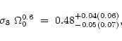
The contours in the
![]() plane in
Fig. 14 closely follow
the curve
plane in
Fig. 14 closely follow
the curve
![]() .
This allows us
to obtain the following measurement of
.
This allows us
to obtain the following measurement of
![]() (from this figure alone):
(from this figure alone):
If we choose a strong prior for ![]() ,
we can constrain
the two parameters separately; for
,
we can constrain
the two parameters separately; for
![]() we get, at the
we get, at the ![]() confidence level:
confidence level:
![]() and
and
![]() for open models
and
for open models
and
![]() and
and
![]() for flat (
for flat (![]() -CDM) models.
However, this result is clearly sensitive to
the prior choosen for
-CDM) models.
However, this result is clearly sensitive to
the prior choosen for ![]() .
In particular, if we use the
relation
.
In particular, if we use the
relation
![]() for a cold dark matter model,
then some extreme combinations of
for a cold dark matter model,
then some extreme combinations of ![]() ,
,
![]() and
and
![]() cannot be ruled out from lensing alone. The degeneracy between
cannot be ruled out from lensing alone. The degeneracy between
![]() and
and ![]() is broken only if we take
is broken only if we take ![]() to lie in
a reasonable interval. Such interval can be motivated by
galaxy surveys for instance, which give
to lie in
a reasonable interval. Such interval can be motivated by
galaxy surveys for instance, which give
![]() at
at ![]() confidence level for the APM
(Eisentsein & Zaldarriaga 2001). For instance the choice
confidence level for the APM
(Eisentsein & Zaldarriaga 2001). For instance the choice
![]() would make
would make
![]() consistent with the data.
The second source of uncertainty comes from the
redshift distribution, kown only approximately. As discussed in Sect. 4.1 and shown in
Fig. 2 we have a rough idea of this distribution, but until we
obtain the information on the photometric or spectroscopic redshifts (which is in progress) we
cannot guarantee a precise cosmological parameter estimation here. Figures 15 and 16 show
the confidence contours as calculated in Fig. 14
but with the two other redshift distributions defined in Sect. 4.1. Despite
the large differences of the distribution, in particular for the number of
galaxies at z>1.5, it is reassuring that the contours are in fact only
slightly modified. The detailed
analysis involving a marginalisation over
consistent with the data.
The second source of uncertainty comes from the
redshift distribution, kown only approximately. As discussed in Sect. 4.1 and shown in
Fig. 2 we have a rough idea of this distribution, but until we
obtain the information on the photometric or spectroscopic redshifts (which is in progress) we
cannot guarantee a precise cosmological parameter estimation here. Figures 15 and 16 show
the confidence contours as calculated in Fig. 14
but with the two other redshift distributions defined in Sect. 4.1. Despite
the large differences of the distribution, in particular for the number of
galaxies at z>1.5, it is reassuring that the contours are in fact only
slightly modified. The detailed
analysis involving a marginalisation over ![]() and over the redshift
distribution of the sources (constrained using photometric redshifts)
is left for a forthcoming study. However,
for the reasonable values of
and over the redshift
distribution of the sources (constrained using photometric redshifts)
is left for a forthcoming study. However,
for the reasonable values of ![]() ,
the degeneracy-breaking for the high
,
the degeneracy-breaking for the high ![]() models
is not affected by the present uncertainty on the redshift distribution
of the sources.
Our result is consistent with the rough guide given by the scaling
models
is not affected by the present uncertainty on the redshift distribution
of the sources.
Our result is consistent with the rough guide given by the scaling
![]() (Jain & Seljak 1997).
(Jain & Seljak 1997).
![\begin{figure}
\par\includegraphics[width=6.4cm,clip]{new_omega_sigma_optimal_z0.7.ps}
\end{figure}](/articles/aa/full/2001/30/aa1091/img157.gif) |
Figure 15:
Likelihood contours as in
Fig. 14, but the source redshift distribution
is assumed to be lower, with
|
![\begin{figure}
\par\includegraphics[width=6.4cm,clip]{new_omega_sigma_optimal_z0.9.ps}
\end{figure}](/articles/aa/full/2001/30/aa1091/img158.gif) |
Figure 16:
Likelihood contours as in
Fig. 14, but the source redshift distribution
is assumed to be higher , with
|
Copyright ESO 2001
![\begin{displaymath}%
{\cal L}={1\over (2\pi)^{n/2} \left\vert\vec{S}\right\vert^...
...t)^T \vec{S}^{-1}\left({\rm {\vec d}-{\vec s}}\right)\right]},
\end{displaymath}](/articles/aa/full/2001/30/aa1091/img124.gif)