4 Statistical measures of shear correlations

4.1 Theory

We summarize the different statistics we shall measure, and how they depend on cosmological models. We concentrate on 2-point statistics and variances, since higher order moments are more difficult to measure, and will be addressed in a forthcoming paper.

Let us assume a normalised source redshift distribution parameterized as:

$$% n(z_{\rm s})={\beta\over z_0 \ \Gamma\left({1+\alpha\over \... ...pha \exp\left[-\left({z_{\rm s}\over z_0}\right)^\beta\right],$$ (2)

with the parameters $(z_0,\alpha ,\beta )=(0.8,2,1.5)$, which is consistent with a limiting magnitude $I_{\rm AB}=24.5$ given by Cohen et al. (2000) (it corresponds to a mean redshift of 1.2). However, in contrast to Cohen et al. (2000) we only have photometric data (in one color), which prevents us from inferring the accurate redshift distribution of our galaxies. The impact of this uncertainty is discussed below. We adopted a simplified approach consisting in looking at the sensitivity of cosmological parameter estimation for three realistic redshift distributions. Therefore in addition to the distribution expressed in Eq. (2) with z₀=0.8, we will consider two other sets, one is $(z_0,\alpha ,\beta )=(0.7,2,1.5)$ and the other $(z_0,\alpha ,\beta )=(0.9,2,1.5)$, which $z_0=0.8\pm 0.1$ (similar to the redshift error quoted in Rhodes et al. 2001), corresponding to an uncertainty in the mean redshift of $\pm 0.15$. The three models are shown in Fig. 2, together with the redshift distribution used in Wilson et al. (2000) corresponding to a magnitude distribution $I\simeq [22.5,23.5]$, slightly brighter than our survey (the thick solid line).

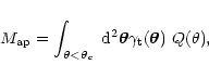
Figure 2: The thin solid line shows our redshift distribution model given by Eq. (2) with $(z_0,\alpha ,\beta )=(0.8,2,1.5)$. Two other models will also be used: one is $(z_0,\alpha ,\beta )=(0.7,2,1.5)$(thin dashed line) and one is $(z_0,\alpha ,\beta )=(0.9,2,1.5)$ (thin dot-dashed line). The thick solid line corresponds to the model used in Wilson et al. (2000) for the $I\simeq [22.5,23.5]$ galaxies. All the distributions are normalised.

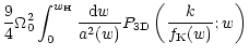
We define the power spectrum of the convergence as (following the notation in Schneider et al. 1998):

 

$$% P_\kappa(k) {9\over 4}\Omega_0^2\int_0^{w_{\rm H}} {{\rm d}w \over a^2(w)} P_{\rm 3D}\left({k\over f_{\rm K}(w)}; w\right)$$ =

$$\times\left[ \int_w^{w_{\rm H}}{\rm d} w' n(w') {f_{\rm K}(w'-w)\over f_{\rm K}(w')}\right]^2,$$ (3)

where $f_{\rm K}(w)$ is the comoving angular diameter distance out to a distance w($w_{\rm H}$ is the horizon distance), and n(w(z)) is the redshift distribution of the sources given in Eq. (2). $P_{\rm 3D}(k)$ is the non-linear mass power spectrum, and k is the 2-dimensional wave vector perpendicular to the line-of-sight. For a top-hat smoothing window of radius $\theta_{\rm c}$, the variance is:

$$% \langle\gamma^2\rangle={2\over \pi\theta_{\rm c}^2} \int_0^\infty~{{\rm d}k\over k} P_\kappa(k) [J_1(k\theta_c)]^2,$$ (4)

where J₁ is the first Bessel function of the first kind.
The aperture mass $M_{\rm ap}$ was introduced in Kaiser et al. (1994):

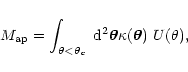$$% M_{\rm ap}=\int_{\theta < \theta_c}~{\rm d}^2\vec{\theta} \kappa(\vec{\theta})~U(\theta),$$ (5)

where $\kappa(\vec{\theta})$ is the convergence field, and $U(\theta)$ is a compensated filter (i.e. with zero mean). Schneider et al. (1998) applied this statistic to the cosmic shear measurements. They showed that the aperture mass variance is related to the convergence power spectrum by:

$$% \langle M_{\rm ap}^2\rangle={288\over \pi\theta_c^4} \int_0^\infty~{{\rm d}k\over k^3} P_\kappa(k) [J_4(k\theta_c)]^2.$$ (6)

$\langle M_{\rm ap}^2\rangle$ can be calculated directly from the shear $\vec{\gamma}$ without the need for a mass reconstruction.

For each galaxy, we define the tangential and radial shear components ( $\gamma_{\rm t}$ and $\gamma_{\rm r}$) with respect to the center of the aperture:

 

$$\gamma_{\rm t} -\gamma_1 \cos(2\phi)-\gamma_2 \sin(2\phi)$$

$$\gamma_{\rm r} -\gamma_2 \cos(2\phi)+\gamma_1 \sin(2\phi),$$ (7)

where $\phi$ is the position angle between the x-axis and the line connecting the aperture center to the galaxy. It is then easy to show that the aperture mass is related to the tangential shear by:

$$% M_{\rm ap}=\int_{\theta < \theta_c}~{\rm d}^2\vec{\theta} \gamma_{\rm t}(\vec{\theta})~Q(\theta),$$ (8)

where the filter $Q(\theta)$ is given from $U(\theta)$:

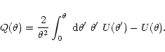$$% Q(\theta)={2\over \theta^2}\int_0^\theta~{\rm d}\theta'~\theta'~U(\theta')-U(\theta).$$ (9)

If $\gamma_{\rm t}$ is replaced by $\gamma_{\rm r}$ in Eq. (8), then the lensing signal vanishes, due to the curl-free property of the shear field (Kaiser et al. 1994). This remarkable property constitutes a test of the lensing origin of the signal. The change from $\gamma_{\rm t}$ to $\gamma_{\rm r}$ can simply be accomplished just by rotating the galaxies by 45 degrees in the aperture (i.e. changing a curl-free field to a pure curl field). Hereafter we call the $M_{\rm ap}$ statistic measured with the 45 degree rotated galaxies the R-mode (R for radial mode), and $\langle M_\perp^2\rangle$ the corresponding variance. It is interesting to note that the R-mode is not expected to vanish if the measured signal is due to spin alignments of galaxies (Crittenden et al. 2000b). Therefore it can be used to constrain the amount of residual systematics as well as the degree of the spin alignment of the galaxies leading to their intrinsic alignment.

From the shear $\vec{\gamma}$ and its projections defined in Eq. (7) we can also define various galaxy pairwise correlation functions related to the convergence power spectrum. Note that the tangential and radial shear projections in what follows are performed using the relative location vector of the pair members, not from an aperture center. The following correlation functions can be defined (Miralda-Escudé 1991; Kaiser 1992):

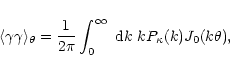$$% \langle\gamma\gamma\rangle_\theta={1\over 2\pi} \int_0^\infty~{\rm d} k~ k P_\kappa(k) J_0(k\theta),$$ (10)

$$% \langle\gamma_{\rm t}\gamma_{\rm t}\rangle_\theta={1\over 4... ...^\infty~{\rm d} k~ k P_\kappa(k) [J_0(k\theta)+J_4(k\theta)],$$ (11)

$$% \langle\gamma_{\rm r}\gamma_{\rm r}\rangle_\theta={1\over 4... ...^\infty~{\rm d} k~ k P_\kappa(k) [J_0(k\theta)-J_4(k\theta)],$$ (12)

where $\theta$ is the pair separation angle. The cross-correlation $\langle\gamma_{\rm t}\gamma_{\rm r}\rangle_\theta$ is expected to vanish for parity reasons (there is no preferred orientation on average).

It is easy to see that the Eqs. (4), (6), (10)-(12) are different ways to measure the same quantity, that is the convergence power spectrum $P_\kappa(k)$. Ultimately the goal is to deproject $P_\kappa(k)$ in order to reconstruct the 3D mass power spectrum from Eq. (3), but this is beyond the scope of this paper. Here we restrict our analysis to a joint detection of these statistics, and show that they are consistent with the gravitational lensing hypothesis. We will also examine the constraints on the power spectrum normalization $\sigma_8$ and the mean density of the universe $\Omega_0$.

4.2 Estimators

Let us now define the estimators we used to measure the quantities given in Eqs. (4), (6), (10)-(12).

The variance of the shear is simply obtained by a cell averaging of the squared shear $\gamma^2(\vec{\theta}_i)$ over the cell index i. An unbiased estimate of the squared shear for the cell i is:

$$% E[\gamma^2(\vec{\theta}_i)]={\displaystyle \sum_{\alpha=1}^... ...vec\theta_l) \over \displaystyle \sum_{k\ne l}^{N_i} w_k w_l},$$ (13)

where w_k is the weight for the galaxy k, and N_i is the number of galaxies in the cell i. The cell averaging over the survey is then an unbiased estimate of the shear variance $\langle \gamma^2\rangle$. However, due to the presence of masked areas (mentioned in Sect. 4.1), some cells may have a very low number of galaxies compared to others. Instead of applying an arbitrary sharp cut off on the fraction of the apertures filled with masks (as in previous works) we decided to keep all the cells, and to weight each of them with the squared sum of the galaxy weights located in the cell. The cell averaging is now defined as:

$$% E[\gamma^2]={\displaystyle \sum_{\rm cells} \left[E[\gamma^... ...{\rm cells} \left[\left(\sum_{k=1}^{N_i} w_k\right)^2\right]},$$ (14)

where i identifies the cell. One potential problem with this procedure is that the sum of the weights is related to the number of objects in the aperture, which is affected by magnification bias, and therefore correlated with the shear signal measured in the same aperture. Fortunately the first non-vanishing contribution of this weighting scheme is a third order effect (of order $1\%$), and is therefore negligible. The advantage is that we can use all cells without wondering about their filling factor, and it naturaly down-weights the cells which contain a large fraction of poorly determined galaxy ellipticities. The weighting scheme of Eq. (14) has been tested against numerical simulation, using a simulated survey with the same survey geometry as our data: it gave unbiased measures of the lensing signal applied to the galaxies.

The $M_{\rm ap}$ statistic is calculated from a similar estimator, although the smoothing window is no longer a top-hat but the Q function defined in Eq. (9). An unbiased estimate of $M_{\rm ap}^2(\vec{\theta}_i)$ in the cell i is:

$$% E[M_{\rm ap}^2(\vec{\theta}_i)]={\displaystyle \sum_{k\ne l... ...ta_k)Q(\theta_l) \over \displaystyle \sum_{k\ne l}^N w_k w_l},$$ (15)

where ${\it e}_{\rm t}^{\rm gal}$ is the tangential galaxy ellipticity, and Q is given by (see Schneider et al. 1998):

$$% Q(\theta)={6\over \pi}\left({\theta\over \theta_c}\right)^2 \left[1-\left({\theta\over \theta_c}\right)^2\right].$$ (16)

The estimation of $\langle M_{\rm ap}^2\rangle$ over the survey is then given by the same expression as in Eq. (14), with $E[\gamma^2(\vec{\theta}_i)]$replaced by $E[M_{\rm ap}^2(\vec{\theta}_i)]$. We emphasize that the this filter probes effective scales $\theta_{\rm c}/5$, and not $\theta_{\rm c}$ (see Fig. 2 in Schneider et al. 1998). Therefore we have to be careful when comparing the signal at different scales between different estimators.

The shear correlation function $\langle\gamma\gamma\rangle_\theta$at separation $\theta$ is obtained by identifying all the pairs of galaxies falling in the separation interval $[\theta-{\rm d}\theta,\theta+{\rm d}\theta]$, and calculating the pairwise shear correlation:

$$% E[\gamma\gamma;\theta]={\displaystyle \sum_{\alpha=1}^2}{\d... ...ec\theta_l) \over \displaystyle \sum_{\rm pairs} w_k w_l}\cdot$$ (17)

The tangential and radial correlation functions $\langle\gamma_{\rm t}\gamma_{\rm t}\rangle_\theta$ and $\langle\gamma_{\rm r}\gamma_{\rm r}\rangle_\theta$are measured also from Eq. (17) by replacing ${\it e}^{\rm gal}$ with ${\it e}_{\rm t}^{\rm gal}$ and ${\it e}_{\rm r}^{\rm gal}$ respectively and dropping the sum over $\alpha$. It is worth noting that the estimators given here are independent of the angular correlation properties of the source galaxies.