We prepared six data subsets (SS1-SS6) out of the 70-day long spectroscopic coverage. Each subset covers approximately one rotation period separated by half a rotation. The successive subsets thus overlap by approximately half of a rotation period but subsets 1, 3, and 5, as well as 2, 4, and 6 represent contiguous stellar rotations. The mid Julian dates for the individual subsets SS1-SS6 are 2450397.980, 2450408.505, 2450417.935, 2450428.410, 2450438.435 and 2450448.365, respectively. Each spectroscopic dataset is supported by simultaneous photometric observations.
Our line-profile inversion code performs a full LTE spectrum synthesis by solving the equation of transfer through a set of Kurucz (1993) model atmospheres, at all aspect angles, and for a given set of chemical abundances. Simultaneous inversions of eight spectral lines, as well as two photometric bandpasses, were carried out using a maximum-entropy regularisation. The number of iterations was set to 15 which proved to be sufficient for a good convergence. The computations were performed on a Sun Ultra-2 workstation at Konkoly Observatory and required 20-30 min of CPU time for each Doppler map. A more detailed description of the TempMap code and additional references regarding our line-profile inversion technique can be found in Rice et al. (1989) and Piskunov & Rice (1993) and previous papers of this series (e.g., Rice & Strassmeier 1998; Strassmeier & Rice 1998).
| Parameter | Value |
| Classification | K1 III |
| Distance (Hipparcos) |
|
| Luminosity, L | 52.5
+14.5-8.2 |
| 2.5 +0.23-0.42 | |
|
|
|
|
|
|
|
|
|
| Inclination, i |
|
| Period,
|
|
| Orbital eccentricity, e | 0.0 |
| Radius, R | 12.3
|
| Microturbulence for Ca,
|
0.7 kms-1 |
| Microturbulence for Fe,
|
1.0 kms-1 |
| Macroturbulence,
|
3.0 kms-1 |
| Chemical abundances | solar (adopted) |
| Element | Ion |
|
||
| Eu | II | 6437.640 | -0.45 | 1.320 |
| Si | I | 6437.703 | -2.35 | 5.863 |
| Ni | I | 6437.992 | -0.75 | 5.389 |
| V | I | 6438.088 | +0.25 | 2.684 |
| Fe | I | 6438.755 | -2.48 | 4.435 |
| Ca | I | 6439.075 | +0.10 | 2.526 |
| Fe | I | 6439.554 | -3.05 | 4.473 |
| Si | I | 6440.566 | -2.48 | 5.616 |
| Fe | I | 6429.071 | -3.41 | 4.294 |
| Co | I | 6429.906 | -2.41 | 2.137 |
| V | I | 6430.472 | -1.00 | 1.955 |
| Fe | I | 6430.844 | -2.00 | 2.176 |
| Ca | I | 6431.099 | -2.61 | 3.910 |
| V | I | 6431.623 | -1.25 | 1.950 |
| Ni | I | 6431.994 | -1.75 | 3.542 |
| Fe | II | 6432.680 | -3.74 | 2.891 |
Table 2 summarizes the astrophysical input parameters for
![]() Gem. We adopt i=60
Gem. We adopt i=60![]() as the most likely inclination
angle. This value was determined by reducing the misfit of the line
profiles as a function of the inclination (for the method see, e.g.,
Rice & Strassmeier 2000 a.o.).
Its uncertainty is estimated from the width of the
as the most likely inclination
angle. This value was determined by reducing the misfit of the line
profiles as a function of the inclination (for the method see, e.g.,
Rice & Strassmeier 2000 a.o.).
Its uncertainty is estimated from the width of the ![]() minimum and
is approximately
minimum and
is approximately ![]() 15
15![]() .
.
![\begin{figure}
\par\includegraphics[angle=0,width=17.1cm,clip]{ms9991f4.eps}
\end{figure}](/articles/aa/full/2001/25/aa9991/img60.gif) |
Figure 4: Fe I 6430-Å images for the six subsets SS1-SS6. Otherwise as in Fig. 3. |
Our best value for the projected rotational velocity,
![]() ,
was determined by minimizing the artificial dark or bright bands in the
Doppler maps that appear if the equatorial velocity,
,
was determined by minimizing the artificial dark or bright bands in the
Doppler maps that appear if the equatorial velocity,
![]() ,
is
either too large or too small, respectively (for more details
see, e.g., Strassmeier et al. 1998, 1999b). Its
uncertainty depends on the S/N ratio and on the "external quality'' of the
spectra (i.e. wavelength calibration, flat fielding, etc.) but also whether
we have a low-gravity giant atmosphere or a high-gravity dwarf atmosphere
and, last but not least, on the spot morphology on the stellar surface. In
case of the K1 giant
,
is
either too large or too small, respectively (for more details
see, e.g., Strassmeier et al. 1998, 1999b). Its
uncertainty depends on the S/N ratio and on the "external quality'' of the
spectra (i.e. wavelength calibration, flat fielding, etc.) but also whether
we have a low-gravity giant atmosphere or a high-gravity dwarf atmosphere
and, last but not least, on the spot morphology on the stellar surface. In
case of the K1 giant ![]() Gem, we estimate an uncertainty of
Gem, we estimate an uncertainty of
![]() 1 kms-1.
1 kms-1.
The minimum radius is computed from the assumption that the rotation is
synchronized to the orbital motion. ![]() becomes then
becomes then
![]()
![]() and, with
and, with
![]() ,
,
![]()
![]() .
This
value is formally below the lower bound of radii found in the literature
for K1 giants (e.g. Gray 1992). The Hipparcos parallax of
.
This
value is formally below the lower bound of radii found in the literature
for K1 giants (e.g. Gray 1992). The Hipparcos parallax of
![]() milli-
milli-
![]() (ESA 1997) and the brightest Vmagnitude observed so far,
(ESA 1997) and the brightest Vmagnitude observed so far,
![]() (see Sect. 3), result
in an absolute visual brightness of +1
(see Sect. 3), result
in an absolute visual brightness of +1
![]() 27 which is almost one magnitude
fainter than tabulated values for K1 giants (Gray 1992). The
radius from the Hipparcos distance and the effective
temperature of 4630 K is 9.3
27 which is almost one magnitude
fainter than tabulated values for K1 giants (Gray 1992). The
radius from the Hipparcos distance and the effective
temperature of 4630 K is 9.3 ![]() (with
B.C.=-0.515; Flower
1996), and is also much smaller than for a fully developed K1
giant and even smaller than our measured minimum radius
(with
B.C.=-0.515; Flower
1996), and is also much smaller than for a fully developed K1
giant and even smaller than our measured minimum radius ![]() .
However, adopting the average surface temperature of
.
However, adopting the average surface temperature of ![]() 4200 K
from our Doppler images as the effective temperature, the radii agree to
within their uncertainties.
O'Neil et al. (1996) obtained a photospheric temperature of 4500 K
and an average spot temperature of 3850 K from measuring titanium oxide
bands contemporaneous with BV photometry. The Hipparcos B-V of 1.118
indicates 4630 K (according to the calibration of Flower 1996). In
any case, this temperature and the bolometric magnitude of +0
4200 K
from our Doppler images as the effective temperature, the radii agree to
within their uncertainties.
O'Neil et al. (1996) obtained a photospheric temperature of 4500 K
and an average spot temperature of 3850 K from measuring titanium oxide
bands contemporaneous with BV photometry. The Hipparcos B-V of 1.118
indicates 4630 K (according to the calibration of Flower 1996). In
any case, this temperature and the bolometric magnitude of +0
![]() 75 suggests
that
75 suggests
that ![]() Gem is beyond the base of the giant branch but not yet in
the helium core-burning phase.
A comparison with the evolutionary tracks from Schaller et al.
(1992) for solar metallicity implies a mass of
Gem is beyond the base of the giant branch but not yet in
the helium core-burning phase.
A comparison with the evolutionary tracks from Schaller et al.
(1992) for solar metallicity implies a mass of
![]()
![]() and an approximate age of 2.8 Gyr.
and an approximate age of 2.8 Gyr.
In this study, we use the Ca I line at 6439 Å and the
Fe I line at 6430 Å as the main mapping lines.
In the (photospheric) temperature range for ![]() Gem, the
Ca I-6439 line is quite temperature sensitive. Therefore,
cooler regions on the stellar surface will appear less pronounced
because inside the spot, i.e. in the regions with lesser continuum
intensity, the Ca line has a relatively large equivalent width and
hence the bump produced by the spot in the Ca profiles appears less
significant. As a result, the Ca I-6439 images provide inferior
"resolution'' compared to the Fe I-6430 images. The iron line
has the advantage that it is less sensitive to the surface temperature
gradient and thus has a smaller equivalent width compared to the Ca line.
Its Doppler images provide thus more surface detail. However, better
fits in the sense of lower
Gem, the
Ca I-6439 line is quite temperature sensitive. Therefore,
cooler regions on the stellar surface will appear less pronounced
because inside the spot, i.e. in the regions with lesser continuum
intensity, the Ca line has a relatively large equivalent width and
hence the bump produced by the spot in the Ca profiles appears less
significant. As a result, the Ca I-6439 images provide inferior
"resolution'' compared to the Fe I-6430 images. The iron line
has the advantage that it is less sensitive to the surface temperature
gradient and thus has a smaller equivalent width compared to the Ca line.
Its Doppler images provide thus more surface detail. However, better
fits in the sense of lower ![]() are obtained for the Ca spectra.
Unfortunately, Fe I-6430 is blended by several relatively strong
metal lines, most notably Fe II at 6432 Å.
are obtained for the Ca spectra.
Unfortunately, Fe I-6430 is blended by several relatively strong
metal lines, most notably Fe II at 6432 Å.
In Table 3, we summarize the atomic parameters that we adopted
for the Ca I-6439 and the Fe I-6430 spectral regions.
By default, solar photospheric abundances were assumed which required
alteration of some of the ![]() values from the line list of Kurucz
(1993) in order to obtain better fits to the spectra.
The effect of an abundance change on the line-profile reconstruction is not
distinguishable from a change of
values from the line list of Kurucz
(1993) in order to obtain better fits to the spectra.
The effect of an abundance change on the line-profile reconstruction is not
distinguishable from a change of ![]() ,
as was noted in previous
papers in this series and quantified in tests with artificial data by Rice &
Strassmeier (2000). Also, abundances from just a single spectral line
can be notoriously uncertain and we chose not to solve for the abundance but
adjust the transition probability instead.
,
as was noted in previous
papers in this series and quantified in tests with artificial data by Rice &
Strassmeier (2000). Also, abundances from just a single spectral line
can be notoriously uncertain and we chose not to solve for the abundance but
adjust the transition probability instead.
![\begin{figure}
\par\includegraphics[angle=0,width=18cm,clip]{ms9991f5.eps}
\end{figure}](/articles/aa/full/2001/25/aa9991/img73.gif) |
Figure 5: a) Average Ca I-6439 map, and b) average Fe I-6430 map. Both maps were obtained from the entire data set spanning 3.6 stellar rotations. |
![\begin{figure}
{\includegraphics[angle=0,height=23.5cm,width=15cm,clip]{ms9991f6.eps} }\end{figure}](/articles/aa/full/2001/25/aa9991/img74.gif) |
Figure 6: Differential maps. Each map is the difference between an individual map in Figs. 3 and 4 and the averge map from Fig. 5. a) for calcium, b) for iron, and c) for the average calcium and iron maps. |
Figures 3 and 4 show the results for the Ca I-6439
and the Fe I-6430 line region, respectively. Six (overlapping) maps
for each wavelength region are obtained (SS1-SS6). None of the maps recovered
a polar cap-like spot, nor any other spots at latitudes higher than 60![]() .
Spots were found mainly along a belt between 30
.
Spots were found mainly along a belt between 30![]() and 60
and 60![]() latitude, but some weaker features were recovered in the low-latitude regions
latitude, but some weaker features were recovered in the low-latitude regions
![]() 30
30![]() from the equator. The main features in the medium-latitude belt
have temperature contrasts of
from the equator. The main features in the medium-latitude belt
have temperature contrasts of
![]() K from the Fe map and 700 K from the Ca map, both values with an rms of
around 50-100 K. The smaller structures in the equatorial regions appear
consistently warmer than these larger features and have
K from the Fe map and 700 K from the Ca map, both values with an rms of
around 50-100 K. The smaller structures in the equatorial regions appear
consistently warmer than these larger features and have
![]() K. Although the calcium line provides a less detailed surface temperature
reconstruction than the iron line due to its intrinsically broader
local line profile, there is reasonable good agreement between the respective
Fe and the Ca maps. We thus conclude that even the weaker equatorial features
are needed by the data and are thus likely real.
K. Although the calcium line provides a less detailed surface temperature
reconstruction than the iron line due to its intrinsically broader
local line profile, there is reasonable good agreement between the respective
Fe and the Ca maps. We thus conclude that even the weaker equatorial features
are needed by the data and are thus likely real.
Several weak warm features with a contrast of
![]() K
are also recovered, mostly at high latitudes, but are related to
dominant cool regions at similar longitudes. We attribute them to the
latitudinal mirroring effect, an artifact of the Doppler-imaging technique
due to the relatively high inclination value of the rotational axis of 60
K
are also recovered, mostly at high latitudes, but are related to
dominant cool regions at similar longitudes. We attribute them to the
latitudinal mirroring effect, an artifact of the Doppler-imaging technique
due to the relatively high inclination value of the rotational axis of 60![]() .
.
Although the photometric data show a changing light curve for the consecutive rotation cycles (see Fig. 1), the changing spot distribution is not obvious from the spectral line profiles. To search for signs of spot evolution during the seventy nights of observation, we first reconstruct the surface temperature distribution from the entire dataset (including all photometric and spectroscopic data in Table 1). The resulting maps in Fig. 5 - one for Ca and one for Fe - are the average surface spot distributions from 3.6 consecutive stellar rotations. A simple visual comparison immediately shows that these average images are generally smoother and have lesser surface detail than the individual images in Figs. 3 and 4. Because the phase coverage is already excellent even for the individual images, we exclude a numerical reason due to the larger number of spectra (it would have the opposite effect than is observed, i.e. with more spectra the features should become better defined). We take this as evidence for spot evolution during the full 3.6 rotation cycles.
Figure 6 shows the spot changes as a function of time by simply plotting the
difference between the individual images (SSi) and the average image as consecutive
differential maps (the top six panels are for the differential Ca maps, the
middle six panels for the differential Fe maps, and the bottom panels for the
average Ca and Fe maps). Notice that the temperature range in these maps is
different to the maps in the previous figures. Further evaluation is then done
by using the reconstructed average map as the input map in the forward problem
and generate an artificial data set, which is then compared with the
observations of the individual data sets. By determining and comparing the
goodness of the line-profile fits from the individual inverse solutions
with the forward computations from the average map, we find that the individual
solutions fit the data on average 22% better than the average image. Table 4
summarizes our goodness of fit statistics.
We calculated a (pseudo) ![]() value for all of our spectra
fitted by either the maps shown in Fig. 4 or the grand-average maps
shown in Fig. 5, defined as
value for all of our spectra
fitted by either the maps shown in Fig. 4 or the grand-average maps
shown in Fig. 5, defined as
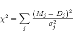 |
(2) |
At this point, we note that the main spotted regions in the average Doppler maps
were also recovered by a fit to the photometric data alone (Sect. 3).
The best fit to the light and color curves was achieved with a spot
temperature contrast of 600![]() 100 K, in agreement with the temperatures
from the Doppler images. The photometric solution also agrees with the Doppler
maps in the sense that no spots were recovered above +60
100 K, in agreement with the temperatures
from the Doppler images. The photometric solution also agrees with the Doppler
maps in the sense that no spots were recovered above +60![]() latitude.
However, the spot at a longitude
of
latitude.
However, the spot at a longitude
of ![]() 240
240![]() (SPOT 3 in Fig. 2) was reconstructed at a
latitude higher by
(SPOT 3 in Fig. 2) was reconstructed at a
latitude higher by ![]() 25
25![]() than in the Doppler maps. We attribute
this difference to the combined effect of sparse sampling of the consecutive
light curves and the mathematical ambiguity that arises from the inversion of
a disk-integrated one-dimensional data set into a surface map.
Being aware of this intrinsic latitude ambiguity, we nevertheless conclude
that the time-series analysis of light curves is a very useful tool
for studying starspot and is supportive of the Doppler-imaging results.
than in the Doppler maps. We attribute
this difference to the combined effect of sparse sampling of the consecutive
light curves and the mathematical ambiguity that arises from the inversion of
a disk-integrated one-dimensional data set into a surface map.
Being aware of this intrinsic latitude ambiguity, we nevertheless conclude
that the time-series analysis of light curves is a very useful tool
for studying starspot and is supportive of the Doppler-imaging results.
| Ca I-6439 | SS1 | SS2 | SS3 | SS4 | SS5 | SS6 |
|
|
4.492 | 5.262 | 5.483 | 3.976 | 2.772 | 3.483 |
|
|
5.747 | 6.206 | 7.103 | 4.735 | 3.312 | 3.331 |
| Fe I-6430 | SS1 | SS2 | SS3 | SS4 | SS5 | SS6 |
|
|
3.575 | 2.981 | 3.822 | 3.699 | 2.886 | 4.804 |
|
|
4.608 | 4.473 | 5.252 | 3.968 | 3.300 | 5.363 |
To isolate a possible surface migration pattern and to obtain a quantitative description of it, we first cross correlate the consecutive Doppler images with each other but for both lines separately (for a detailed description of the method see Collier Cameron (2001) and previous papers in this series). We only cross-correlate the phase independent contiguous images, i.e., Corr{SS1/SS3}, Corr{SS2/SS4}, Corr{SS3/SS5}, and Corr{SS4/SS6} so that any cross-talk from a signature in the same line profile is excluded. This restricts the time resolution to one stellar rotation. The resulting cross-correlation-function maps (ccf-maps) for the Ca and Fe lines are displayed in Figs. 7a and b, respectively.
In most cases a coherent latitude dependency of the correlation signal is seen
in maps from both spectral lines. Nevertheless, the results in Fig. 7 are
inconclusive. Clear equatorial deceleration within an approximately ![]()
![]() range around the equator is seen in Corr{SS2/SS4} and Corr{SS3/SS5}, no
convincing pattern seems to be evident in Corr{SS4/SS6}, and Corr{SS1/SS3}
recovers a pattern with a longitudinal shift direction that appears mostly reversed
with respect to the other three correlation maps in Fig. 7.
We also cross-correlated the two images with the largest time span in between,
i.e. Corr{SS1/SS6}, but the ambiguity remained.
range around the equator is seen in Corr{SS2/SS4} and Corr{SS3/SS5}, no
convincing pattern seems to be evident in Corr{SS4/SS6}, and Corr{SS1/SS3}
recovers a pattern with a longitudinal shift direction that appears mostly reversed
with respect to the other three correlation maps in Fig. 7.
We also cross-correlated the two images with the largest time span in between,
i.e. Corr{SS1/SS6}, but the ambiguity remained.
We then computed an average cross-correlation function from all individual ccfs
shown in Fig. 7 and searched for a correlation peak in each latitude strip
(for a description of the procedure see e.g. Paper V by Weber & Strassmeier
1998). These peaks are then fitted with a
bi-quadratic differential rotation law between the
![]() latitude range (i.e. the most reliable part of our Doppler maps). Despite
the very weak statistical significance, it suggests a solar-like acceleration
in two nearly symmetric bands around the equator for
latitude range (i.e. the most reliable part of our Doppler maps). Despite
the very weak statistical significance, it suggests a solar-like acceleration
in two nearly symmetric bands around the equator for ![]() Gem
(the
Gem
(the ![]() for the bi-quadratic fit was 9.31 and 10.22 was achieved for a
quadratic fit with just one term, while we got 17.55 for a linear fit,
i.e. the same longitudinal shift for all latitudes).
Nevertheless, we consider
this as too weak a detection. Obviously, a simple interpretation with a
latitude-dependent surface differential rotation pattern is not
straightforward from our data. We believe our analysis is hampered by two
facts. Firstly, the spot pattern may not have changed enough during the time
of our observations in order to resolve a coherent differential-rotation
signature and, secondly, the cross correlations may have been masked by
individual spot evolution.
for the bi-quadratic fit was 9.31 and 10.22 was achieved for a
quadratic fit with just one term, while we got 17.55 for a linear fit,
i.e. the same longitudinal shift for all latitudes).
Nevertheless, we consider
this as too weak a detection. Obviously, a simple interpretation with a
latitude-dependent surface differential rotation pattern is not
straightforward from our data. We believe our analysis is hampered by two
facts. Firstly, the spot pattern may not have changed enough during the time
of our observations in order to resolve a coherent differential-rotation
signature and, secondly, the cross correlations may have been masked by
individual spot evolution.
Copyright ESO 2001
![\begin{figure}
\par\includegraphics[angle=0,width=17.1cm,clip]{ms9991f3.eps}
\end{figure}](/articles/aa/full/2001/25/aa9991/img59.gif)
![\begin{figure}
\includegraphics[angle=0,width=18cm,clip]{ms9991f7.eps}
\end{figure}](/articles/aa/full/2001/25/aa9991/img85.gif)