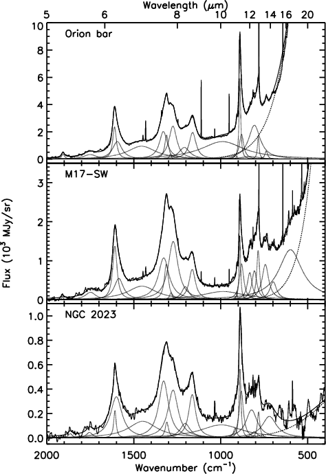
The continuum below the AIBs shows a clear evolution from NGC 2023 to the Orion Bar (see Fig. 1): continuous emission of hot, small (radii of a few 10 to 100 Å, Désert et al. 1990) grains between 10 and 20 $\mu$ m is prominent in M17-SW and the Orion Bar whereas this is completely absent in NGC 2023. This is a consequence of the stronger flux and harder radiation field in the Orion Bar which heats up these small grains.

The 6.2 and 7.7 $\mu$ m bands do not vary much with respect to each other whereas they do relative to the 3.3, 8.6 and 11.3 $\mu$ m AIBs. Such variations cannot be interpreted as the result of different emission temperature distributions of PAHs (obtained with different size distributions and/or radiation field effective temperature). In fact, the 3.3 $\mu$ m-band is dominated by the emission of small (hot) PAHs while the 11.3 $\mu$ m-band is contributed to by larger (cold) PAHs (Schutte et al. 1993): thus, changing the PAH temperature distribution cannot explain why the 11.3 $\mu$ m-band varies along with the 3.3 $\mu$ m-band. Instead, modifications of the physical state of PAHs have to be invoked. Theoretical (de Frees et al. 1993; Pauzat et al. 1995, 1997; Langhoff 1996) and laboratory (Szczepanski & Vala 1993; Hudgins et al. 1994; Hudgins & Allamandola 1995; Hudgins & Sandford 1998) studies showed that ionized species have stronger C-C bands. On the other hand, dehydrogenated PAHs have weaker C-H bands (Pauzat et al. 1995, 1997). As we show in Sect. 4.4.1, the weaker C-H band emission in M17-SW can be explained if the hydrogenation fraction is significantly reduced.

Moreover, the AIB profiles show little spectral substructure even though most AIBs are fully resolved in our SWS data (the resolving power is $\lambda / \Delta\lambda =$ 200 to 500). A direct comparison of the spectra displayed in Fig. 1 shows that the position and width of the major, simple AIBs (at 3.3, 6.2, 8.6 and 11.3 $\mu$ m) are roughly the same. The decomposition of the spectra we discuss below primarily aims at quantifying this comparison and also at disentangling in a systematic way the profile of a given AIB from the other bands, as well as from the underlying continuum due to hot small grains.

Boulanger et al. (1998b) showed that the AIBs in CAM-CVF data can be decomposed into Lorentz profiles and a linear underlying continuum. It must be emphasized, however, that the AIBs are barely resolved in the CAM-CVF data (in particular the 6.2, 8.6 and 11.3 $\mu$ m bands, see Table 2 in Boulanger et al. 1998b and Fig. 3 of Cesarsky et al. 2000). The SWS data at high spectral resolution presented here do not suffer from this limitation. The use of a Lorentzian band shape implicitly assumes that the AIB profiles arise from the intrinsic width of molecular transitions and/or resonances in small solid particles (e.g. , Bohren & Huffman 1983).

In the current paradigm, the AIBs result from the superposition of many vibrational bands produced by a population of interstellar PAHs with a wide range of sizes (molecules containing a few tens to a few hundred carbon atoms, Désert et al. 1990; Schutte et al. 1993). In this respect, laboratory and theoretical studies on small PAH species teach us that the band shapes (position and width) of vibrational transitions (i) depend on the temperature of the molecule (Joblin et al. 1995) and, (ii) vary from one species to another (in particular, the position of the vibrational bands depends on the size and symmetry of the molecule: Szczepanski & Vala 1993; Hudgins & Allamandola 1995 and 1998; Joblin et al. 1995; Langhoff 1996). The observed AIBs may actually result from a combination of these two effects. Elaborating on these studies, variability in the AIBs (changing band ratios, presence of substructure in the band profiles) from different interstellar sightlines is predicted as a consequence of a changing PAH population and/or different exciting radiation fields. Specifically, the position and width of individual bands are expected to vary by a few to several tens of cm_1 from one species to another and/or as a result of different emission temperatures. Some changes in the AIB profiles have been observed towards H II regions and reflection nebulae (Roelfsema et al. 1996; Verstraete et al. 1996; Cesarsky et al. 2000a; Uchida et al. 2000; Peeters et al. 2000 in preparation). The case of the general (bright) interstellar medium is covered below with a quantitative comparison of the AIB profiles.

In this work, rather than establish the "final'' AIB profile parameters, we aim at comparing on the same footing the individual AIB profiles under different excitation conditions. We have therefore decomposed the present spectra into Lorentz profiles and a modified blackbody as underlying continuum. We restricted ourselves to the minimum number of Lorentz profiles required in order to produce a reasonable overall fit and a good representation of every individual AIB.

We used a classical gradient-expansion algorithm with analytical partial derivatives and performed the fit in the wavenumber space ( $x=1/\lambda$ in cm_1) over the 2.4-25 $\mu$ m wavelength range. In addition to the Lorentz profiles, the underlying continuum is fitted simultaneously. For the latter, we took a modified blackbody with an emissivity law proportional to x, the temperature and peak brightness of which were the free parameters. The same set of fit parameters was used for all objects. Such a set was first fixed on the M17-SW spectrum which has a high signal-to-noise ratio and a good feature-to-continuum contrast. To fit the 2.4-25 $\mu$ m spectrum, twenty Lorentz profiles were necessary. Then, the parameter values of the Lorentz profiles and of the continuum in M17-SW were used as input to fit the other AIB spectra: very good fits were obtained by first relaxing the Lorentz amplitudes and blackbody continuum parameters, suggesting a complete and robust decomposition of the AIB spectrum. After adjusting the amplitudes, the profile (position and width) and continuum parameters were fine-tuned, simultaneously, over restricted spectral ranges. The centroids, widths and amplitudes of the Lorentzian fits to the main AIBs are given in Table 2. Our fit to the 5-25 $\mu$ m-AIB spectrum is shown in Fig. 2. The blackbody component of this decomposition is consistent with the emission of warm dust in the mid-infrared and in particular its exponential decay (the Wien tail of the blackbody). The observed strong variability of the 20 $\mu$ m-continuum flux (very weak in NGC 2023 whereas strong in M17-SW and the Orion Bar) then reflects the varying temperature of the warm dust component. As can be seen in Fig. 2, the underlying continuum contributes little below the AIBs. On the other hand, additional, colder blackbody, type continua are required to fit the full SWS spectra out to 45 $\mu$ m.

We note that broad bands are required at about 1000 and 1450 cm_1 in order to explain the continuum between the AIBs. These bands may not be associated with the AIBs but, for simplicity, we assumed their profiles to be Lorentzian. Their parameters are not well constrained in our decomposition: the sole requirement is that the corresponding profiles are broad enough to reproduce the smooth continuum observed in these spectral regions. The fitted profiles of the neighbouring AIBs are somewhat sensitive to the widths adopted for the 1000 and 1450 cm_1 bands: for instance, if the full width at half maximum (FWHM) of the 1450 cm_1 band is increased from 200 to 300 cm_1, the 6.2 $\mu$ m-band has its FWHM reduced by 2.5 cm_1 and its position redshifted by 0.8 cm_1. In order to coherently compare the AIB profiles, we have fixed the width of these broad bands: namely, ${\it FWHM} = 300$ cm_1 for the 1000 cm_1-band and ${\it FWHM} = 200$ cm_1 for the 1450 cm_1-band. At this stage, we can point out that combinations of PAH vibrational modes have been predicted to accumulate between 1000 and 2000 cm_1 in a broad structure (Bernard et al. 1989).

**Table 2:** Fit parameters of the AIB Lorentz profiles.
AIB	NGC 2023	M17-SW	Orion Bar

11.3 $\mu$ m	888.6 ¹	889.9	889.7
	20.8 ²	17.8	14.2
	877 ³	2292	7241
Core	889.3	890.2	889.9
	13.1	10.1	10.9
	564	1644	5928
Red wing	881.9	880.3	880.5
	29.6	30.4	30.0
	384	915	1820
8.6 $\mu$ m	1164.0	1163.8	1161.5
	49.3	44.6	48.0
	355	780	1957
7.8 $\mu$ m	1274.2	1273.5	1275.1
	70.2	67.6	54.2
	392	1494	2417
7.6 $\mu$ m	1309.9	1312.6	1311.3
	22.9	28.6	25.6
	130	912	1760
7.5 $\mu$ m	1328.1	1327.8	1329.7
	68.2	74.5	55.9
	466	1074	2022
6.2 $\mu$ m	1608.1	1607.7	1609.7
	48.6	42.6	38.9
	550	1748	3428
Core	1608.5	1608.6	1610.5
	17.1	30.0	25.5
	224	1376	2369
Red wing	1600.5	1586.2	1594.9
	80.0	64.4	64.8
	338	546	1291
3.3 $\mu$ m	3041.8	3039.1	3040.0
	43.0	38.8	40.4
	98	171	834

Also noteworthy is that two Lorentzians are required to correctly reproduce the red wing asymmetry of the 1609 cm_1 (6.2 $\mu$ m) and 890 cm_1 (11.3 $\mu$ m) bands: these components are labelled "core'' and "red wing'' in Table 2. The feature centered around 1300 cm_1 (the classical "7.7 $\mu$ m-band'') shows 3 sub-peaks at about 1273, 1310 and 1328 cm_1. In the following, we will call the narrow 1310 cm_1 peak the "7.6 $\mu$ m-band'' while the broader 1273 and 1328 cm_1 components will be dubbed the "7.8'' and "7.5 $\mu$ m-bands'' respectively. The observed 1310 cm_1-feature has a narrow core and a broad blue wing which demands another component at 1328 cm_1. A Lorentzian is also required around 1204 cm_1 ( ${\it FWHM} \sim 70$ cm_1) to fill the gap between the 7.8 and the 8.6 $\mu$ m-features. In the case of Orion this band shifts to 1209 cm_1 in order to reproduce the pronounced and extended blue wing of the 8.6 $\mu$ m-band.

In Fig. 3 we show the profile and fit of the 3.3 $\mu$ m band. The band shape is also Lorentzian and the continuum has the same functional form as in the 5-25 $\mu$ m region. In other words, we fitted the 2.4-25 $\mu$ m continuum with a single blackbody component.

The decomposition presented above is not unique: we also tried to use a multicomponent power-law continuum (A/x³ + B/x² + C/x + D with $x=1/\lambda$ and where A,B,C and D are constant parameters) below the AIBs from 2.4 to 16 $\mu$ m. Such a continuum gives a notable contribution below the AIBs, in particular, it replaces completely the 1000 cm_1 broad band. However, a multicomponent power-law continuum has no straightforward physical interpretation and it cannot describe the strong rise of the spectrum beyond 16 $\mu$ m observed in M17-SW and the Orion Bar. Nor can it accommodate the weak 20 $\mu$ m-flux in NGC 2023. In any case, comparing the fits obtained with the two types of continua (power-law and blackbody), we found the positions and widths of the main AIBs characterized in Table 2 to vary by less than 1.6 and 4 cm_1 respectively in a given object. Finally, using gaussian band shapes for the AIBs, we got as good a decomposition (see also Boulanger et al. 1998b): yet the continuum under the AIBs was stronger and more structured because of the weaker profile wings. We believe that the fit quality does not preclude any band profile: in fact, the SWS AIB spectrum is so rich that there are always enough parameters in the fit to accomodate any choice of band profile.

$\begin{figure} {\epsfig{figure={ms10317_f2.eps},width=6.7cm} } \end{figure}$

Figure 2: The decomposition of the AIB spectra between 5 and 25 $\mu$ m. The resolving power ( $\lambda /\Delta \lambda$ ) of the data is 200 for NGC 2023 and 500 for M17-SW and the Orion Bar. Each Lorentz component is represented by a dotted line, the underlying continuum by a dashed line. The full fit is the solid line.

We have thus determined in a coherent way the position and width of the strong, well-delineated AIBs at 3.3, 6.2, 7.6, 8.6 and 11.3 $\mu$ m with an accuracy of 0.8 and 2 cm_1 respectively. Inspection of Table 2 shows that there are significant variations in the width of the 6.2 and 11.3 $\mu$ m-bands (9.7 and 6.6 cm_1 respectively) as well as in the position of the 3.3 and 7.6 $\mu$ m-bands (2.7 cm_1 in both cases). However, all these variations come within the accuracy range given above when the values of NGC 2023 are excluded. In this latter object, the poorer signal-to-noise ratio and resolving power (see Fig. 1 and Figs. 8 to 11) has degraded the band profiles: this is probably why some AIB parameters are singular in NGC 2023. On the other hand, we find that the position of the 8.6 $\mu$ m-band varies by 2.5 cm_1 (Table 2) and that most of this variation is due to a redshift in the Orion Bar spectrum. As noted above, the 8.6 $\mu$ m-band in this object has an extended blue wing: this spectral change is related to the redshift of the band itself. This result may point to the more profound modifications seen in this spectral range by Roelfsema et al. (1996) and Verstraete et al. (1996) towards more excited regions.

$\begin{figure} {\epsfig{figure={ms10317_f3.eps},width=6.7cm} } \end{figure}$

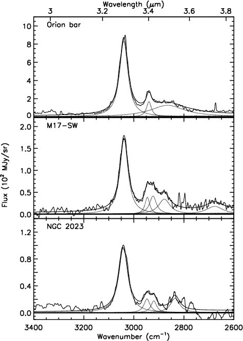Figure 3: Same as Fig. 2 in the region of the 3.3 $\mu$ m AIB. Note that the continuum has the same functional form than that already seen in Fig. 2. In the Orion Bar spectrum, the Pf $\delta$ hydrogen recombination line clearly visible on the top of the 3.3 $\mu$ m-band was masked to perform the fit. The Pf $\gamma$ at 3.74 $\mu$ m and Pf $\epsilon$ at 3.04 $\mu$ m lines can also be seen in emission in the Orion Bar spectrum.

From the above discussion, we conclude that most AIB profiles (except the 8.6 $\mu$ m-AIB in the Orion Bar) do not vary within the accuracy of our spectral decomposition. At 3.3 $\mu$ m, a similar result was already obtained by Tokunaga et al. (1991) who compared the band profile of planetary nebulae and H II regions (their Type 1 profile) with excitation conditions ( $T_{\rm eff}$ and $\chi$ ) similar to that of our sample (see Table 1). Roche et al. (1996) confirmed this result on a larger, lower-excitation sample of planetary nebulae. Similarly, Witteborn et al. (1989) showed that the 11.3 $\mu$ m-band profile is rather stable. Furthermore, the observed smoothness and invariance of the AIBs across a wide range of excitation conditions appears difficult to reconcile with the variability expected from laboratory results.

Having performed this mathematical parameterization of the SWS spectra, we are now able to extract the individual AIB profiles and to compare them in different objects and to model predictions. Yet, what is the physical meaning of this spectral decomposition? We have chosen Lorentzian band shapes and we represented most AIBs (except the 7.7 $\mu$ m) with one or two Lorentz profiles: this implicitly assumes that the AIBs arise from a few vibrational bands common to many PAHs and that most of the bandwidth arises from a single carrier. The invariance and smoothness of the AIBs is then naturally explained (Boulanger et al. 1998b). To verify this interpretation of the AIBs, the band parameters of Table 2 can be compared directly to laboratory or theoretical studies on relevant PAHs (large molecules containing more than 50 C-atoms as argued by Boulanger et al. 1998b). But there are other ways to look at the interstellar AIB spectrum which do not result in Lorentzian bandshapes. For instance, simulations of astronomical spectra based on recent laboratory studies of small PAHs (Allamandola et al. 1999) have shown that the AIB spectrum may be decomposed by assigning a multiplicity of (species dependent) vibrational bands to each AIB. Another possibility to interpret the AIB spectrum is based on the laboratory work of Joblin et al. (1995) which shows that the vibrational bands of PAHs are broadened and redshifted as the temperature of the molecule is raised. In this picture, the profile of a vibrational band from a single molecule with a given internal energy has a Lorentz shape (the intrinsic profile) which only depends on the temperature of the molecule (and not on the species). The observed AIBs are then interpreted as the superposition of many Lorentz profiles corresponding to all the possible temperatures reached by a population of PAHs.

In the next section, devoted to modelling, we adopt and detail this latter view of the AIB spectrum. In this context, using the relationship between bandwidth and temperature established by Joblin et al. (1995), we note that the width of the observed 3.3 $\mu$ m-band (40 cm_1) is well explained if the emitting PAH has a temperature of about 1000 K. Such emission temperatures are in good agreement with what is expected for interstellar PAHs emitting during temperature fluctuations (see Sect. 4). Using the present spectral decomposition of the SWS data, we can now extract the individual AIB profiles and compare them to the predictions of a PAH emission model that uses the best available laboratory data on PAHs.

3 The observed AIB profiles