3 Data acquisition and reduction

The HI data presented in this paper were obtained with the Westerbork Synthesis Radio Telescope (WSRT) between 1991 and 1996. The integration times varied between $1 \times 12^{\rm h}$ and $5 \times 12^{\rm h}$ depending on the required signal-to-noise. The angular resolution at the center of the cluster is $12^{\prime\prime}\times16^{\prime\prime}$ or $1.08\times 1.44$ kpc at the adopted distance of 18.6 Mpc. The FWHM of the primary beam is 37.4 arcminutes or 202 kpc. As a result, often more than one galaxy was mapped in a single field of view. The observed bandwidth was either 2.5 or 5 MHz, depending on the width of the global profiles. The observations of the NGC 3992-group and the NGC 4111-group required a broad frequency band of 5 MHz and at the same time also sufficient velocity resolution for the dwarf systems. To comply with the correlator restrictions, those two fields were observed only in one polarization (XX) which allowed for a velocity resolution of 10 km s^-1 but resulted in less sensitivity. During the earlier measurements an on-line Hanning taper was applied but this tapering was abandoned later to obtain the highest possible velocity resolution. The various obtained velocity resolutions (dependent on the correlator restrictions) were 5, 8, 10, 20 or 33 km s^-1, corresponding to typical rms-noise levels of respectively 3.1, 1.9, 2.9, 1.6 and 1.0 mJy beam^-1 for a single 12h observation at the highest angular resolution. The data of NGC 4013 were kindly made available by R. Bottema who studied this system in great detail (Bottema 1996 and references therein).

More details on the observational parameters for each field are tabulated in the atlas along with the data. What follows is a brief description of the reduction procedures.

 

 

Table 1: All galaxies in the Ursa Major cluster brighter than M^b,i(B)=-16.8 and more inclined than 45 degrees

Name	RA	Dec	Galactic		Type	D25(B)	PA	1-b/a	$i_{\rm opt}$	$i_{\rm adopt}$	S.B.	[BH]
	(1950)		Long.	Lat.		($^\prime$)	($^\circ$)		($^\circ$)	($^\circ$)		mag	mag
(1)	(2)	(3)	(4)	(5)	(6)	(7)	(8)	(9)	(10)	(11)	(12)	(13)	(14)
Galaxies with fully analyzed HI data:
U6399	11 20 35.9	51 10 09	152.08	60.96	Sm	2.40	140	0.72	79	$75\pm2$	LSB	0.00	0.07
U6446	11 23 52.9	54 01 21	147.56	59.14	Sd	2.27	200	0.38	54	$51\pm3$	LSB	0.00	0.07
N3726	11 30 38.7	47 18 20	155.38	64.88	SBc	5.83	194	0.38	54	$53\pm2$	HSB	0.01	0.07
N3769	11 35 02.8	48 10 10	152.72	64.75	SBb	2.97	150	0.69	76	$70\pm2$	HSB	0.01	0.10
U6667	11 39 45.3	51 52 32	146.27	62.29	Scd	3.43	88	0.88	90	$89\pm1$	LSB	0.00	0.07
N3877	11 43 29.3	47 46 21	150.72	65.96	Sc	5.40	36	0.78	84	$76\pm1$	HSB	0.01	0.10
N3893	11 46 00.2	48 59 20	148.15	65.23	Sc	3.93	352	0.33	49	$49\pm2$	HSB	0.02	0.09
N3917	11 48 07.7	52 06 09	143.65	62.79	Scd	4.67	257	0.76	82	$79\pm2$	LSB	0.01	0.09
N3949	11 51 05.5	48 08 14	147.63	66.40	Sbc	2.90	297	0.38	54	$55\pm2$	HSB	0.03	0.09
N3953	11 51 12.4	52 36 18	142.21	62.59	SBbc	6.10	13	0.50	62	$62\pm1$	HSB	0.01	0.13
N3972	11 53 09.0	55 35 56	138.85	60.06	Sbc	3.43	298	0.72	79	$77\pm1$	HSB	0.00	0.06
U6917	11 53 53.1	50 42 27	143.46	64.45	SBd	3.17	123	0.46	59	$56\pm2$	LSB	0.03	0.12
U6923	11 54 14.4	53 26 19	140.51	62.06	Sdm	1.97	354	0.58	68	$65\pm2$	LSB	0.00	0.12
U6930i	11 54 42.3	49 33 41	144.54	65.51	SBd	3.00	39	0.14	32	$31\pm3$	LSB	0.05	0.13
N3992	11 55 00.9	53 39 11	140.09	61.92	SBbc	6.93	248	0.44	58	$56\pm2$	HSB	0.01	0.13
U6940f	11 55 12.4	53 30 46	140.17	62.06	Scd	0.83	135	0.72	79	$75\pm3$	LSB	0.00	0.12
U6962i	11 55 59.5	43 00 44	154.08	71.05	SBcd	2.33	179	0.20	38	$37\pm3$	HSB	0.00	0.09
N4010	11 56 02.0	47 32 16	146.68	67.36	SBd	4.63	65	0.88	90	$89\pm1$	LSB	0.00	0.11
U6969	11 56 12.9	53 42 11	139.70	61.96	Sm	1.50	330	0.69	76	$76\pm2$	LSB	0.01	0.13
U6973	11 56 17.8	43 00 03	153.97	71.10	Sab	2.67	40	0.61	70	$71\pm3$	HSB	0.00	0.09
U6983	11 56 34.9	52 59 08	140.27	62.62	SBcd	3.20	270	0.34	50	$49\pm1$	LSB	0.01	0.12
N4051	12 00 36.4	44 48 36	148.88	70.08	SBbc	5.90	311	0.34	50	$49\pm3$	HSB	0.00	0.06
N4085	12 02 50.4	50 37 54	140.59	65.17	Sc	2.80	255	0.76	82	$82\pm2$	HSB	0.01	0.08
N4088	12 03 02.0	50 49 03	140.33	65.01	Sbc	5.37	231	0.63	71	$69\pm2$	HSB	0.01	0.09
N4100	12 03 36.4	49 51 41	141.11	65.92	Sbc	5.23	344	0.71	77	$73\pm2$	HSB	0.03	0.10
N4102	12 03 51.3	52 59 22	138.08	63.07	SBab	3.00	38	0.44	58	$56\pm2$	HSB	0.01	0.09
N4157	12 08 34.2	50 45 47	138.47	65.41	Sb	6.73	63	0.83	90	$82\pm3$	HSB	0.02	0.09
N4183	12 10 46.5	43 58 33	145.39	71.73	Scd	4.77	346	0.86	90	$82\pm2$	LSB	0.00	0.06
N4217	12 13 21.6	47 22 11	139.90	68.85	Sb	5.67	230	0.74	80	$86\pm2$	HSB	0.00	0.08
N4389	12 23 08.8	45 57 41	136.73	70.74	SBbc	2.50	276	0.34	50	$50\pm4$	HSB	0.00	0.06
Galaxies with partially analyzed HI data:
N3718	11 29 49.9	53 20 39	147.01	60.22	Sa	7.53	195	0.58	68	$69\pm3$	HSB	0.00	0.06
N3729	11 31 04.9	53 24 08	146.64	60.28	SBab	2.80	164	0.32	48	$49\pm3$	HSB	0.00	0.05
U6773	11 45 22.1	50 05 12	146.89	64.27	Sm	1.53	341	0.47	60	$58\pm3$	LSB	0.00	0.07
U6818	11 48 10.1	46 05 09	151.76	67.78	Sd	2.20	77	0.72	79	$75\pm3$	LSB	0.00	0.09
U6894	11 52 47.3	54 56 08	139.52	60.63	Scd	1.67	269	0.84	90	$83\pm3$	LSB	0.00	0.06
N3985	11 54 06.4	48 36 48	145.94	66.27	Sm	1.40	70	0.37	53	$51\pm3$	HSB	0.05	0.11
N4013	11 55 56.8	44 13 31	151.86	70.09	Sb	4.87	245	0.76	88	$90\pm1$	HSB	0.00	0.07
U7089	12 03 25.4	43 25 18	149.90	71.52	Sdm	3.50	215	0.81	90	$80\pm3$	LSB	0.00	0.07
U7094	12 03 38.5	43 14 05	150.14	71.70	Sdm	1.60	39	0.64	72	$70\pm3$	LSB	0.00	0.06
N4117	12 05 14.2	43 24 17	149.07	71.72	S0	1.53	21	0.56	67	$68\pm3$	LSB	0.00	0.06
N4138	12 06 58.6	43 57 49	147.29	71.40	Sa	2.43	151	0.37	53	$53\pm3$	HSB	0.00	0.06
N4218	12 13 17.4	48 24 36	138.88	67.88	Sm	1.17	316	0.40	55	$53\pm3$	HSB	0.00	0.07
N4220	12 13 42.8	48 09 41	138.94	68.13	Sa	3.63	140	0.69	76	$78\pm3$	HSB	0.00	0.08
Galaxies with confused HI data:
1135+48	11 35 09.2	48 09 31	152.71	64.77	Sm	1.23	114	0.69	76	$73\pm3$	LSB	0.01	0.10
N3896	11 46 18.6	48 57 10	148.10	65.29	Sm	1.60	308	0.33	49	$48\pm3$	LSB	0.02	0.09
Not observed or too little HI content:
N3870	11 43 17.5	50 28 40	147.02	63.75	S0a	1.13	17	0.31	47	$48\pm3$	HSB	0.00	0.07
N3990	11 55 00.3	55 44 13	138.25	60.04	S0	1.47	40	0.50	62	$63\pm3$	HSB	0.00	0.07
N4026	11 56 50.7	51 14 24	141.94	64.20	S0	4.37	177	0.74	80	$84\pm3$	HSB	0.04	0.10
N4111	12 04 31.0	43 20 40	149.53	71.69	S0	4.47	150	0.78	84	$90\pm3$	HSB	0.00	0.06
U7129	12 06 23.6	42 01 08	151.00	72.99	Sa	1.27	72	0.31	47	$48\pm3$	HSB	0.00	0.06
N4143	12 07 04.6	42 48 44	149.18	72.40	S0	2.60	143	0.46	59	$60\pm3$	HSB	0.00	0.06
N4346	12 21 01.2	47 16 15	136.57	69.39	S0	3.47	98	0.67	75	$77\pm3$	HSB	0.00	0.06

 

 

Table 2: Photometrics of all galaxies in the UMa cluster brighter than M^b,i(B)=-16.8 and more inclined than 45 degrees

Name	$m^{\rm tot}_{B}$	$m^{\rm tot}_{R}$	$m^{\rm tot}_{I}$	$m^{\rm tot}_{K^\prime}$	WR,Ii	AiB	AiR	AiI	$A^i_{K^\prime}$	Mb,iB	Mb,iR	Mb,iI	$M^{b,i}_{K^\prime}$	Db,i25
	mag	mag	mag	mag	$\rm {km~s}^{-1}$	mag	mag	mag	mag	mag	mag	mag	mag	($^\prime$)
(1)	(2)	(3)	(4)	(5)	(6)	(7)	(8)	(9)	(10)	(11)	(12)	(13)	(14)	(15)
Galaxies with fully analyzed HI data:
U6399	14.33	13.31	12.88	11.09	172	0.47	0.36	0.27	0.06	-17.56	-18.44	-18.77	-20.33	1.84
U6446	13.52	12.81	12.58	11.50	174	0.18	0.14	0.10	0.02	-18.08	-18.72	-18.90	-19.88	2.07
N3726	11.00	9.97	9.51	7.96	331	0.34	0.25	0.20	0.05	-20.76	-21.67	-22.07	-23.45	5.32
N3769	12.80	11.56	10.99	9.10	256	0.67	0.50	0.39	0.09	-19.32	-20.35	-20.80	-22.35	2.34
U6667	14.33	13.11	12.63	10.81	167	0.74	0.58	0.43	0.10	-17.83	-18.87	-19.18	-20.65	2.18
N3877	11.91	10.46	9.72	7.75	335	1.06	0.78	0.62	0.15	-20.60	-21.73	-22.29	-23.76	3.95
N3893	11.20	10.19	9.71	7.84	382	0.31	0.23	0.18	0.04	-20.55	-21.45	-21.86	-23.56	3.67
N3917	12.66	11.42	10.85	9.08	276	0.87	0.64	0.51	0.12	-19.65	-20.63	-21.05	-22.40	3.48
N3949	11.55	10.69	10.28	8.43	321	0.33	0.24	0.20	0.05	-20.22	-20.96	-21.31	-22.98	2.66
N3953	11.03	9.66	9.02	7.03	446	0.60	0.43	0.35	0.08	-21.05	-22.20	-22.74	-24.41	5.38
N3972	13.09	11.90	11.34	9.39	264	0.76	0.56	0.44	0.11	-19.08	-20.05	-20.48	-22.08	2.62
U6917	13.15	12.16	11.74	10.30	224	0.31	0.23	0.18	0.04	-18.63	-19.49	-19.84	-21.10	2.84
U6923	13.91	12.97	12.36	11.04	160	0.28	0.22	0.16	0.04	-17.84	-18.67	-19.20	-20.36	1.67
U6930i	12.70	11.71	11.39	10.33	231	0.08	0.06	0.05	0.01	-18.86	-19.78	-20.07	-21.04	2.98
N3992	10.86	9.55	8.94	7.23	547	0.56	0.40	0.33	0.08	-21.18	-22.28	-22.80	-24.21	6.27
U6940f	16.45	15.65	15.44	13.99	50	0.00	0.00	0.00	0.00	-15.02	-15.77	-15.96	-17.37	0.64
U6962i	12.88	11.88	11.42	10.11	327	0.16	0.11	0.09	0.02	-18.72	-19.64	-20.06	-21.27	2.26
N4010	13.36	12.14	11.55	9.22	254	1.20	0.89	0.70	0.17	-19.30	-20.17	-20.55	-22.31	2.97
U6969	15.12	14.32	14.04	12.58	117	0.20	0.17	0.11	0.02	-16.56	-17.28	-17.48	-18.80	1.19
U6973	12.94	11.26	10.53	8.23	364	0.71	0.52	0.42	0.10	-19.21	-20.67	-21.28	-23.23	2.21
U6983	13.10	12.27	11.91	10.52	221	0.21	0.16	0.12	0.03	-18.58	-19.31	-19.61	-20.87	2.99
N4051	10.98	9.88	9.37	7.86	308	0.28	0.21	0.17	0.04	-20.71	-21.72	-22.18	-23.54	5.45
N4085	13.09	11.87	11.28	9.20	247	0.78	0.58	0.46	0.11	-19.12	-20.11	-20.57	-22.27	2.08
N4088	11.23	10.00	9.37	7.46	362	0.74	0.54	0.43	0.10	-20.95	-21.94	-22.45	-24.00	4.40
N4100	11.91	10.62	10.00	8.02	386	0.97	0.70	0.57	0.14	-20.51	-21.49	-21.97	-23.48	4.07
N4102	12.04	10.54	9.93	7.86	393	0.46	0.34	0.27	0.07	-19.86	-21.20	-21.73	-23.57	2.69
N4157	12.12	10.60	9.88	7.52	399	1.40	1.02	0.82	0.20	-20.72	-21.83	-22.33	-24.04	4.64
N4183	12.96	11.99	11.51	9.76	228	1.01	0.76	0.59	0.14	-19.46	-20.16	-20.46	-21.74	3.13
N4217	12.15	10.62	9.84	7.61	381	1.05	0.76	0.62	0.15	-20.33	-21.54	-22.16	-23.90	4.29
N4389	12.56	11.33	10.87	9.12	212	0.20	0.15	0.12	0.03	-19.05	-20.21	-20.63	-22.27	2.31
Galaxies with partially analyzed HI data:
N3718	11.28	9.95	9.29	7.47	476	0.77	0.55	0.45	0.11	-20.90	-21.99	-22.54	-24.00	6.30
N3729	12.31	10.94	10.30	8.60	296	0.25	0.18	0.15	0.03	-19.34	-20.62	-21.22	-22.78	2.60
U6773	14.42	13.61	13.15	11.23	112	0.09	0.08	0.05	0.01	-17.09	-17.87	-18.28	-20.14	1.35
U6818	14.43	13.62	13.15	11.70	151	0.39	0.31	0.22	0.05	-17.40	-18.10	-18.46	-19.71	1.69
U6894	15.27	14.31	14.00	12.40	124	0.37	0.31	0.21	0.05	-16.51	-17.39	-17.59	-19.01	1.13
N3985	13.25	12.26	11.81	10.19	180	0.18	0.14	0.10	0.02	-18.39	-19.30	-19.69	-21.19	1.29
N4013	12.44	10.79	9.95	7.68	377	1.10	0.80	0.64	0.15	-20.08	-21.40	-22.07	-23.83	3.61
U7089	13.73	12.77	12.36	11.11	138	0.42	0.34	0.24	0.05	-18.11	-18.96	-19.26	-20.30	2.46
U7094	14.74	13.70	13.22	11.58	76	0.00	0.00	0.00	0.00	-16.67	-17.69	-18.16	-19.78	1.29
N4117	14.05	12.47	11.81	9.98	285	0.00	0.00	0.00	0.00	-17.36	-18.92	-19.57	-21.38	1.29
N4138	12.27	10.72	10.09	8.19	374	0.36	0.26	0.21	0.05	-19.50	-20.93	-21.50	-23.22	2.22
N4218	13.69	12.83	12.41	10.83	150	0.15	0.12	0.09	0.02	-17.88	-18.68	-19.06	-20.55	1.06
N4220	12.34	10.79	10.03	8.36	399	0.94	0.68	0.55	0.13	-20.03	-21.29	-21.91	-23.13	2.85
Galaxies with confused HI data:
1135+48	14.95	14.05	13.61	11.98	111	0.17	0.15	0.09	0.02	-16.67	-17.51	-17.88	-19.40	0.97
N3896	13.75	12.96	12.47	11.35	83	0.00	0.00	0.00	0.00	-17.69	-18.45	-18.92	-20.01	1.49
Not observed or too little HI content:
N3870	13.67	12.71	12.16	10.73	127	0.08	0.06	0.04	0.01	-17.83	-18.74	-19.26	-20.64	1.06
N3990	13.53	12.08	11.36	9.54	...	0.00	0.00	0.00	0.00	-17.89	-19.31	-20.02	-21.82	1.28
N4026	11.71	10.25	9.57	7.65	...	0.00	0.00	0.00	0.00	-19.74	-21.16	-21.82	-23.71	3.32
N4111	11.40	9.95	9.25	7.60	...	0.00	0.00	0.00	0.00	-20.01	-21.44	-22.13	-23.76	3.24
U7129	14.13	12.80	12.19	...	...	0.08	0.06	0.04	0.01	-17.36	-18.65	-19.23	...	1.19
N4143	12.06	10.55	9.84	7.86	...	0.00	0.00	0.00	0.00	-19.35	-20.83	-21.54	-23.50	2.30
N4346	12.14	10.69	9.96	8.21	...	0.00	0.00	0.00	0.00	-19.27	-20.70	-21.42	-23.15	2.75

 

 

Table 3: A comparison of the widths and integrated fluxes from the present WSRT survey and from the literature

	This study					Literature
Name	W20	$\pm$	Res.	$\int S{\rm d}v$	$\pm$	W20	$\pm$	Res.	$\int S{\rm d}v$	$\pm$	Ref.
	- - - km s-1 - - -			- Jy km s-1 -		- - - km s-1 - - -			- Jy km s-1 -
(1)	(2)	(3)	(4)	(5)	(6)	(7)	(8)	(9)	(10)	(11)	(12)
U6399	188.1	1.4	8.3	10.5	0.3	178	20	22	10.1	1.9	1
U6446	154.1	1.0	5.0	40.6	0.5	162	10	22	45.9	4.1	1
N3718(c)	492.8	1.0	33.2	140.9	0.9	480	10	5.5	84.9	26.4	1
						508m	..	33	120	...	8	$^{\rm WSRT}$
N3726	286.5	1.6	5.0	89.8	0.8	290	10	5.5	83.9	10.8	1
N3729 $^{\rm noSD}$	270.8	1.5	33.2	5.5	0.3	...	..	..	...	...	..
						279m	..	33	25?	...	8	$^{\rm WSRT}$
N3769i	265.3	6.7	8.3	62.3	0.6	276	20	7.4	44.1	4.2	2
U6667	187.5	1.4	5.0	11.0	0.4	210	20	22	11.6	2.2	1
N3877	373.4	5.0	33.2	19.5	0.6	352	10	22	24.8	5.6	1
U6773	110.4	2.3	8.3	5.6	0.4	118	8	22	5.6	0.7	6
N3893(c)	310.9	1.0	5.0	69.9	0.5	313	8	22	85.3	5.1	1
N3917	294.5	1.9	8.3	24.9	0.6	284	10	22	21.9	4.7	1
U6818	166.9	2.3	8.3	13.9	0.2	168	15	22	14.8	2.1	1
N3949	286.5	1.4	8.3	44.8	0.4	289	10	22	42.7	5.4	1
N3953l	441.9	2.4	33.1	39.3	0.8	423	10	22	41.0	3.9	1
U6894	141.8	1.1	8.3	5.8	0.2	159	20	7.4	5.1	1.7	2
N3972	281.2	1.4	8.3	16.6	0.4	270	15	22	14.0	2.6	1
U6917	208.9	3.2	8.3	26.2	0.3	211	10	22	31.5	4.1	1
N3985	160.2	3.7	8.3	15.7	0.6	168	..	22	14.1	0.9	5
U6923	166.8	2.4	10.0	10.7	0.6	175	15	22	8.2	2.9	1
						189m	15	41.4	15.6	...	12	$^{\rm VLA}$
U6930	136.5	0.5	8.3	42.7	0.3	145	8	22	38.2	3.5	1
N3992l	478.5	1.4	10.0	74.6	1.5	480	10	22	81.2	5.3	1
						507m	15	41.4	79.9	...	12	$^{\rm VLA}$
U6940	59.3	3.8	10.0	2.1	0.3	226	..	22	7.0	1.0	3
						121m	15	41.4	2.7	...	12	$^{\rm VLA}$
N4013	425.0	0.9	33.0	41.5	0.2	403	10	22	33.8	3.7	1
U6962(c)	220.3	6.6	8.3	10.0	0.3	...	..	22	21.6	4.4	1
						235	..	33	9.2	1.0	4	$^{\rm WSRT}$
N4010	277.7	1.0	8.3	38.2	0.3	281	10	22	38.1	3.4	1
U6969c	132.1	6.4	10.0	6.1	0.5	146	..	13.2	6.0	1.4	3
						159m	15	41.4	6.9	...	12	$^{\rm VLA}$
U6973 $^{\rm noSD}$	367.8	1.8	8.3	22.9	0.2	...	..	..	...	...	..
						408	..	33	18.3	1.2	4	$^{\rm WSRT}$
U6983	188.4	1.3	5.0	38.5	0.6	205	10	22	36.2	4.4	1
N4051l	255.4	1.8	5.0	35.6	0.8	274	15	22	43.4	3.3	1
N4085c	277.4	6.6	19.8	14.6	0.9	299	20	7.4	23.3	2.5	2
						311m	..	33	24!	...	13	$^{\rm WSRT}$
N4088(c)	371.4	1.7	19.8	102.9	1.1	381	8	22	109.2	6.4	1
						378m	..	33	128!	...	13	$^{\rm WSRT}$
U7089(c)	156.7	1.7	10.0	17.0	0.6	162	10	22	17.8	2.2	1
						176	..	33.4	18.9	...	11	$^{\rm WSRT}$
N4100	401.8	2.0	19.9	41.6	0.7	420	20	22	54.0	7.3	1
U7094c	83.7	1.7	10.0	2.9	0.2	112	8	22	6.0	0.6	6
						153?	..	33.4	2.5	...	11	$^{\rm WSRT}$
N4102	349.8	2.0	8.3	8.0	0.2	327	20	7.4	10.3	2.1	2
N4117 $^{\rm noSD}$	289.4	7.5	10.0	6.9	1.1	...	..	..	...	...	..
						314	..	33.4	5.3	...	11	$^{\rm WSRT}$
N4138	331.6	4.5	19.9	19.2	0.7	354m	30	6.8	16	...	14
						340	5	5.2	20.6	0.3	7	$^{\rm VLA}$
N4157(c),l	427.6	2.2	19.9	107.4	1.6	436	10	22	123.9	9.5	1
N4183	249.6	1.2	8.3	48.9	0.7	258	10	22	49.6	5.3	1
N4218	138.0	5.0	8.3	7.8	0.2	160	20	13	5.7	0.9	9
N4217	428.1	5.1	33.2	33.8	0.7	426	20	22	51.8	7.2	1
N4220	438.1	1.3	33.1	4.4	0.3	382m	..	11	3.3	...	10
N4389	184.0	1.5	8.3	7.6	0.2	174	20	7.4	7.6	0.8	2

 

Table 3: continued. Notes

(c):	the authors suggest possible confusion with a dwarf companion.
c:	flagged by the authors as confused with near companion.
l:	large correction factor (>1.20) applied for primary beam flux attenuation.
i:	flagged by the authors as possibly interacting.
$^{\rm noSD}$:	no useful single dish profile available due to obvious confusion.
m:	line width directly measured from the published HI profile.
!:	the integrated flux as quoted by the author is a factor 2 larger than is quoted by
	any other source. Therefore, half the integrated flux was adopted from this source.
$^{\rm WSRT}$:	synthesis observation with the WSRT.
$^{\rm VLA}$:	synthesis observation with the VLA.
References:	1: Fisher & Tully (1981)	8: Schwarz (1985)
	2: Appleton & Davies (1982)	9: Thuan & Martin (1981)
	3: Richter & Huchtmeier (1991)	10: Magri (1994)
	4: Oosterloo & Shostak (1993)	11: Van der Burg (1987)
	5: Huchtmeier & Richter (1986)	12: Gottesman et al. (1984)
	6: Schneider et al. (1992)	13: Van Moorsel (1983)
	7: Jore et al. (1996)	14: Grewing & Mebold (1975)

The raw UV-data were calibrated, interactively flagged and Fast Fourier Transformed (FFT) using the NEWSTAR software developed at the NFRA in Dwingeloo. The UV points were weighted according to the local density of points in the UV plane and a Gaussian baseline taper was applied with a FWHM of 2293 (m) which attenuates the longest baseline by 50%. To deal with the frequency dependent antenna pattern, five antenna patterns were calculated for each data cube at a regular frequency separation thoughout the bandpass. Pixel sizes of 5 arcsec in RA and $\frac{5}{\sin(\delta)}$ arcsec in declination ensure an adequate sampling of the synthesized beam, $12^{\prime\prime}\times 12^{\prime\prime}/\sin(\delta)$.

After the FFT, the datacubes and antenna patterns were further processed using the Groningen Image Processing SYstem (GIPSY). Several channels at the low and high velocity end of the bandpass were discarded because of their higher noise. As a result, there are 110 or 53 usable channels for a bandpass of 2.5 or 5 MHz respectively, except for the N3992 and N4111 fields which had 110 channels across a 5 MHz bandpass. All datacubes were smoothed to lower angular resolutions of $30^{\prime\prime}\times30^{\prime\prime}$ and $60^{\prime\prime}\times60^{\prime\prime}$. This facilitates the detection of extended low level HI emission and the identification of the "continuum'' channels which are free from line emission.

3.1 The radio continuum emission

The channels free from HI emission were averaged and the resulting continuum map was subtracted from all channels in the data cube. The residuals of the frequency dependent grating rings were only a minor fraction of the noise in the channels containing the line emission. The dirty continuum maps were cleaned (Högbom 1974) down to 0.3$\sigma$. The clean-components were restored with a Gaussian beam of similar FWHM as the synthesized beam. When radio continuum emission from a galaxy was detected, its continuum flux was determined from the cleaned continuum map. In cases of no detection, an upper limit for extended emission was derived by calculating the rms scatter in the flux values obtained by integrating the noise in each of fifteen elliptical areas enclosed by the 25th mag blue isophote and positioned at various emission-free regions in the map.

3.2 The HI channel maps and the global HI profiles

At all three spatial resolutions, the regions of HI emission were defined by the areas enclosed by the 2$\sigma$ contours in the "dirty'' 60 $^{\prime\prime}$ resolution maps. Grating rings and noise peaks above this level were removed manually. The selected regions were enlarged by moving their boundaries 1 armin outwards to account for possible emission in the sidelobes. The resulting masks vary from channel to channel in shape, size and position due to the rotation of the HI disk. These masks defined the regions that were cleaned down to 0.3$\sigma$ at all three spatial resolutions.

The clean-components were restored with a Gaussian beam of similar FWHMas the synthesized beam. The global HI profiles were derived by determining the primary beam corrected flux in each cleaned region. Since the size and shape of the clean masks vary as a function of velocity, the uncertainty in the flux densities at each velocity in the global HI profile varies as well. The noise on the global HI profile was determined by projecting each clean mask at nine different line-free positions in a channel map and integrating over each of them.

For further analysis, each profile was divided up in three equal velocity bins in which the peak fluxes $F^{\rm peak}_{\rm low}$, $F^{\rm peak}_{\rm mid}$and $F^{\rm peak}_{\rm high}$ were determined for the low, middle and high velocity bin respectively. These three peak fluxes were then used to classify a global profile shape according to:
Double peaked: $F^{\rm peak}_{\rm low}>F^{\rm peak}_{\rm mid}<F^{\rm peak}_{\rm high}$
Gaussian: $F^{\rm peak}_{\rm low}<F^{\rm peak}_{\rm mid}>F^{\rm peak}_{\rm high}$
Distorted: $F^{\rm peak}_{\rm low}<F^{\rm peak}_{\rm mid}<F^{\rm peak}_{\rm high}$
                or $F^{\rm peak}_{\rm low}>F^{\rm peak}_{\rm mid}>F^{\rm peak}_{\rm high}$
Boxy: $F^{\rm peak}_{\rm low}\approx F^{\rm peak}_{\rm mid}\approx F^{\rm peak}_{\rm high}$.
In case of a double peaked profile, the peak fluxes on both sides were considered separately when calculating the 20% and 50% levels. In all other cases, the overal peak flux was used. The four velocities $V_{\rm low}^{20\%}$, $V_{\rm low}^{50\%}$, $V_{\rm high}^{50\%}$ and $V_{\rm high}^{20\%}$ corresponding to these 20% and 50% levels were determined by linear interpolation between the data points, going from the center outward. In the few cases of non-monotonically decreasing edges, this procedure tends to slightly underestimate the widths. The widths are calculated according to

$W_{20}=V_{\rm high}^{20\%}-V_{\rm low}^{20\%}\ {\rm and} \ W_{50}=V_{\rm high}^{50\%}-V_{\rm low}^{50\%}$.

The systemic velocity is calculated according to

$V_{\rm sys}=0.25(V_{\rm low}^{20\%}+V_{\rm low}^{50\%}+V_{\rm high}^{50\%}+V_{\rm high}^{20\%}).$

Because in interferometric measurements some flux may be lost due to the missing short baselines, it is useful to compare the widths and flux densities from the WSRT profiles with those from published single dish observations. However, a meaningful comparison requires that the profile widths are all corrected in the same way for instrumental broadening. In general, the widths that are published by various authors were corrected for instrumental broadening using nearly as many different methods. Therefore, the published line widths had to be de-corrected first to ensure a uniformly applied correction. The de-corrected widths and integrated HI fluxes from the literature are compiled in Cols. (7)-(11) of Table 3 along with the results from this study in Cols. (2)-(6).
Column (1) gives the NGC or UGC numbers.
Columns (2, 3) and (7, 8) give the widths of the global profiles at the 20% levels and the formal uncertainties.
Columns (4) and (9) give the velocity resolutions of the observations.
Columns (5, 6) and (10, 11) contain the integrated HI fluxes derived from the global profiles.
Column (12) provides the references to the literature sources.
In case the authors suggest that the single dish profile of a particular galaxy may be confused and synthesis data on that galaxy do exist, these synthesis data are included as well and used in the following comparison. However, first it will be explained how the observed linewidths are corrected for the different instrumental resolutions.

3.2.1 Correcting ${\mathsfsl {W}}_{\mathsf 20}$ for instrumental broadening

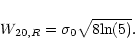
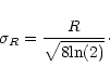
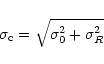
The most widely used method to correct for broadening of the global HI profiles due to a finite instrumental velocity resolution was provided by Bottinelli et al. (1990). For the widths at the 20% and 50% levels of the peak flux they advocate the following linear relations:

$W_{20,R}=W_{20}-\delta W_{20}=W_{20}-0.55R$
$W_{50,R}=W_{50}-\delta W_{50}=W_{50}-0.13R$

where W₂₀ is the observed linewidth and W_20,R is the linewidth corrected for the instrumental velocity resolution R in km s^-1. This empirical prescription is based on comparing linewidths obtained at different resolutions.

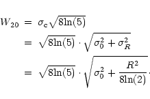
However, the correction method applied here deviates from Bottinelli et al.'s method and is based on more analytic considerations. It is easy to imagine that both edges of an intrinsic global profile, when chopped off at their peaks and glued together, approximate a Gaussian with dispersion $\sigma_0$. The width at the 20% level of this "true'' Gaussian is then given by

$$W_{20,R} = \sigma_0\sqrt{8 \mbox{ln}(5)}.$$

A spectral Hanning smoothing was applied to most of the WSRT observations presented in this paper. This smoothing function can also be approximated by a Gaussian with a FWHM equal to the instrumental velocity resolution R and has a dispersion $\sigma_R$

$$\sigma_{R} = \frac{R}{\sqrt{8 \mbox{ln}(2)}}\cdot$$

The dispersion $\sigma_{\rm c}$ of the convolved observed Gaussian is then given by

$$\sigma_{\rm c} = \sqrt{ \sigma_0^2 + \sigma_R^2 }$$

and the 20% line width of this convolved or observed Gaussian is given by

$$\begin{eqnarray*}W_{20} & = & \sigma_{\rm c} \sqrt{8\mbox{ln}(5)} \\ & = & \sqr... ...{ln}(5)}\cdot\sqrt{\sigma_0^2 + \frac{R^2}{8\mbox{ln}(2)} }\cdot \end{eqnarray*}$$

So, at the 20% level, the intrinsic width W_20,R is broadened to W₂₀ by $\delta{W}$ given by

$$\begin{eqnarray*}\delta{W}_{20} & = & {W}_{20} - {W}_{20,R} \\ & = & \sqrt{8\mb... ...sqrt{1 + \frac{(R/\sigma_0)^2}{8\mbox{ln}(2)} } - 1 \right]\cdot \end{eqnarray*}$$

The broadening $\delta W_{20}$ does not only depend on the instrumental resolution R but also on the steepness of the slopes of the edges of the profile, expressed by $\sigma_0$. Fitting Gaussians to the edges of a profile yields $\sigma_{\rm c}$ from which $\sigma_0$ can be calculated given the known value of $\sigma_R$. The equation above can be rewritten using $\sigma_{\rm c}$ instead which results in

$$\delta{W}_{20} = \sigma_{\rm c}\sqrt{8\mbox{ln}(2)}\left(\fra... ...sqrt{1-\frac{(R/\sigma_{\rm c})^2}{8\mbox{ln}(2)}}\right]\cdot$$

However, no Gaussians were fitted to the edges of the new WSRT profiles. Instead it is assumed that the slopes of the edges of the profiles are more or less determined by the turbulent motion of the gas with a canonical velocity dispersion of $\sigma_0=10~{\rm km}\, {\rm s}^{-1}$. This results in

$$\delta{W}_{20} = 35.8\cdot\left[\sqrt{1 + \left(\frac{R}{23.5}\right)^2} - 1 \right]$$

and similarly for the 50% level

$$\delta{W}_{50} = 23.5\cdot\left[\sqrt{1 + \left(\frac{R}{23.5}\right)^2} - 1 \right]\cdot$$

The differences between Bottinelli et al.'s linear presciption and our corrections ( $\Delta\delta{W}=\delta{\rm W}^{Bot}-\delta{W}^{\rm our}$) are only minor and tabulated below for typical instrumental resolutions of the WSRT.

level	$\Delta\delta W$
	- - - - - R (km s-1) - - - - -
	5.0	8.3	16.5	19.9	33.1
20%	2.0	2.4	1.2	0.2	-7.8
50%	0.2	-0.3	-3.1	-4.7	-12.8

The larger differences occur for the poorest resolutions at which only the broadest profiles were observed. Consequently, the differences are a negligible fraction of the line widths.

Figure 1 shows the comparison of the widths and integrated fluxes derived from the new WSRT global profiles and those from the literature. There are no significant systematic differences. The unweighted average difference in widths is $-0.9 \pm 2.1~{\rm km}\, {\rm s}^{-1}$ with a rms scatter of 14 km s^-1. The unweighted average difference in integrated flux is $4.7\pm 3.5$ percent with a rms scatter of 25 percent. It can therefore be concluded that on average the WSRT results are in excellent agreement with the results from single dish observations.

Figure 1: A comparison of the present WSRT results with pre-existing single dish and synthesis data from the literature

3.3 The total HI maps

As a next step, the total integrated HI maps were constructed from the cleaned datacubes. The clean-masks were used to define the regions with HI emission. Outside these regions, the pixels were set to zero and all the channels containing a non-zero area were added to build up the integrated column density map. This was then corrected for attenuation by the primary beam. Although the advantage of this procedure is a higher signal-to-noise ratio at a certain pixel in the HI map, the disadvantage is that the noise is no longer uniform across the map. As a result, the 3$\sigma$-contour level in an integrated HI map is not defined. Signal-to-noise maps have been made, however, using the prescription outlined in Appendix A and the average pixel value of all pixels with $2.75<(\frac{S}{N})<3.25$ was determined. This average value was adopted as the "3$\sigma$'' level for the column density.

3.4 The radial HI surface density profiles

The integrated column density maps were used to derive the radial HI surface density profiles by azimuthally averaging in concentric ellipses. The orientations and widths of the ellipses were the same as those of the projected tilted rings fitted to the HI velocity field (see Sect. 3.6.1). In the case of a warp with overlapping ellipses, the flux in the overlapping regions was proportionally assigned to each ellipse. The azimuthal averaging was done separately for the receding and approaching halves of each tilted ring to reveal possible asymmetries. Pixels in the HI map without any measured signal were set to zero. Finally, the entire radial profile was scaled by the total HI mass as derived from the global HI profile. No attempt was made to correct the profiles for the effect of beam smearing.

This method for extracting the surface density profiles from integrated HI maps breaks down for nearly edge-on systems; the highly inclined annuli with large major axis diameters could still pick up some flux along the minor axis due to beam smearing. In such cases, Lucy's (1974) iterative deprojection scheme as adapted and developed by Warmels (1988b) might be preferable.

Due to the complex noise structure of the integrated HI map, no attempt was made to estimate the errors on the radial HI surface density profiles.

3.5 The HI velocity fields

The HI data cubes were smoothed to velocity resolution of $\approx$ $19~{\rm km}\, {\rm s}^{-1}$ in order to obtain a good spectral signal-to-noise ratio. HI velocity fields were then constructed by fitting single Gaussians to the velocity profiles at each pixel. Initial estimates for the fits were given by the various moments of the profiles determined over the velocity range covered by the masks. Only those fits were accepted for which 1) the central velocity of the fitted Gaussian lies inside the masked volume, 2) the amplitude is larger than five times the rms noise in the profile and 3) the uncertainty in the central velocity is smaller than $\frac{1}{3}$ the velocity resolution.

Due to projection effects and beam smearing, the velocity profiles in highly inclined systems and in the central regions of galaxies may deviate strongly from a Gaussian shape. The exact shape depends on the spatial and kinematic distribution of the gas within a synthesized beam. Fitting single Gaussians to these usually skewed profiles results in an underestimate of the rotational velocity at that position. As a consequence, the gradients in the velocity field become shallower. There are several methods to correct for the effects of beam smearing. In the present cases, however, the signal-to-noise was in general too low to allow a useful application of these methods, and, since only a small number of systems were recognized as seriously affected, the HI velocity fields were not corrected for the effects of beam smearing.

3.6 Rotation curves

The rotation curves were derived in two ways; 1) by fitting tilted-rings to the velocity fields (Begeman 1987) and 2) by estimating the rotational velocities by eye from the position-velocity diagrams.

3.6.1 Using the velocity fields

The determination of the rotation curves from the velocity fields was done in three steps by fitting tilted rings to the velocity field (see Begeman 1987, 1989). The widths of the rings were set at $\frac{2}{3}$ of the width of the synthesized beam (i.e. $10^{\prime\prime}$, $20^{\prime\prime}$ or $40^{\prime\prime}$).

First, the systemic velocity and the dynamical center were determined. In this first step the inclination and position angles were the same for each ring and kept fixed at the values derived from the optical images. The systemic velocity, center and rotational velocity were fitted for each ring. All the points along the tilted ring were considered and weighted uniformly. In general, no significant trend as a function of radius could be detected for the systemic velocity and center. The adopted values were calculated as the average of all rings.

Second, the systemic velocity and center of rotation were kept fixed for each ring while the position angle, inclination and rotational velocity were fitted. All the points along the tilted ring were considered but weighted with cos($\theta$) where $\theta$ is the angle in the plane of the galaxy measured from the receding side. Hence, points along the minor axis have zero weight. While the position angle can be determined accurately, the inclination and rotational velocity are rather strongly correlated for inclinations below 60 degrees and above 80 degrees (Begeman 1989). As a result, the fitted inclinations can vary by a large amount from one ring to another. However, a possible trend in the inclination with radius due to a central bar or a warp can be detected. A change in inclination angle often goes together with a change in the more accurately determined position angle.

Third, the rotational velocity was fitted again for each ring while keeping the systemic velocity, center of rotation, inclination and position angle fixed. Again, all the points along the tilted ring were considered but weighted with cos($\theta$). The fixed values for the inclination and position angles were determined in the second step by averaging the solutions over all the rings or fixing a clear trend. For nearly edge-on galaxies, the inclinations determined in the second step were often overruled by higher values based on the clear presence of a dust lane (e.g. N4010, N4157, N4217) or the very thin distribution of gas in the column density maps (e.g. U6667). However, uncertainty in the inclinations of nearly edge-on systems does not significantly influence the amplitude of the rotational velocity.

The results of this 3-step procedure were used to construct a model velocity field. This model was subtracted from the actual observed velocity field to yield a map of the residual velocities. In some cases (e.g. N3769, N4051, N4088) this residual map shows significant systematic residuals, indicative of non-circular motion or a bad model fit due to a noisy observed velocity field. As a further check, the derived rotation curve is projected onto the position-velocity maps along the major and minor axis.

The errors on the inclination and position angles and the rotational velocity are formal errors. They do not include possible systematic uncertainties due to, for instance, the beam smearing.

3.6.2 Using the position-velocity diagrams

It has already been remarked (see Sect. 3.5) that beam smearing affects the determination of the velocity fields, especially in the central regions of galaxies and in highly inclined disks. As a consequence, the rotation curves derived from such velocity fields are underestimated as one can see from their projection on the XV-maps. In order to overcome this problem, the rotation curves were derived directly from the major axis XV-maps in a manner similar to that used for edge-on systems (cf. Sancisi & Allen 1979). This was done by two independent human neural networks trained to estimate the maximum rotational velocity from the asymmetric velocity profiles, taking into account the instrumental band- and beam-widths and the random gas motions. This was done for both the receding and approaching side of a galaxy. The rotation curves were then deprojected (also accounting for possible warps) by using the same position and inclination angles as fixed in the third step described in the previous section. In general, the average rotation curves derived from the XV-diagrams are in reasonable agreement with those obtained by the tilted ring fits. As expected, significant differences can only be noted for galaxies which are highly inclined or have a steeply rising rotation curve.

From the XV-diagrams it is clear that many galaxies have kinematic asymmetries in the sense that the rotation curve often rises more steeply on one side of a galaxy than on the other side (e.g. N3877, N3949). The rotation curves as derived from the velocity fields and XV-diagrams are tabulated in Table 4 for the approaching and receding parts separately. The adopted changes in inclination and position angles of N3718 and N4138 are motivated in the notes on the atlas pages of these galaxies. The uncertainties quoted in Table 4 are not 1-sigma Gaussian errors but rather reflect fiducial velocity ranges, based on the position-velocity diagrams.

 

 

Table 4: Rotation curves derived from velocity fields and XV-diagrams

Rad.	$V^{\rm app}_{\rm rot}$	$\pm$		$V^{\rm rec}_{\rm rot}$	$\pm$		$V^{\rm ave}_{\rm rot}$	i	PA
( $^{\prime\prime}$)	- - - km s-1 - - -			- - - km s-1 - - -			km s-1	($^\circ$)	($^\circ$)
U6399
10	25	12	7	25	10	7	25	75	141
20	44	10	7	49	7	7	46	75	141
30	61	12	7	61	7	5	61	75	141
40	70	7	5	69	5	5	70	75	141
50	77	7	5	78	3	5	78	75	141
60	82	10	5	84	5	5	83	75	141
70	84	5	5	-	-	-	84	75	141
80	86	5	5	-	-	-	86	75	141
90	88	5	5	-	-	-	88	75	141
U6446
10	39	8	8	23	10	10	31	51	188
20	49	8	8	61	8	10	55	51	188
30	57	5	5	65	5	8	61	51	188
40	63	5	5	65	5	8	64	51	188
50	69	8	5	65	5	5	67	51	188
60	71	5	5	70	5	5	70	51	188
70	75	5	5	72	5	5	74	51	188
80	79	8	5	77	5	5	78	51	188
90	81	8	5	81	5	5	81	51	188
100	81	5	5	80	5	5	81	51	188
110	81	5	5	82	5	5	81	51	189
120	82	8	5	83	5	8	82	51	191
131	82	8	5	84	5	8	83	51	193
142	83	8	8	86	8	8	85	51	195
153	83	8	8	86	8	8	84	51	197
164	82	11	11	85	8	11	83	51	199
176	80	11	11	-	-	-	80	51	201
N3726
40	112	10	7	92	12	10	102	53	195
60	131	7	7	119	10	10	125	53	195
80	144	5	5	146	7	10	145	53	195
100	156	5	5	172	5	7	164	53	195
120	154	7	7	171	5	7	162	53	195
140	155	7	5	166	7	7	160	53	195
160	152	7	7	159	5	7	156	53	195
183	145	10	7	148	5	5	147	57	188
256	157	8	8	159	6	6	158	72	180
316	169	9	12	-	-	-	169	75	179
344	169	9	12	-	-	-	169	75	179
373	167	15	15	-	-	-	167	75	179
N3769
20	89	13	10	86	20	10	88	70	149
40	103	10	8	109	13	10	106	70	149
60	112	8	8	119	8	8	116	70	149
80	120	8	8	130	8	10	125	70	149
100	123	5	8	129	5	8	126	70	149
120	124	5	8	122	5	8	123	70	150
141	120	5	5	115	8	8	118	70	152
166	120	8	10	110	8	10	115	70	155
196	122	14	17	-	-	-	122	70	158
364	121	10	10	-	-	-	121	70	167
396	118	10	10	-	-	-	118	70	167
426	113	11	11	-	-	-	113	70	168
U6667
10	27	5	5	27	7	7	27	89	89
20	43	2	2	47	5	5	45	89	89
30	55	5	5	59	7	5	57	89	89
40	64	2	5	74	5	5	69	89	89

 

Table 4: continued

Rad.	$V^{\rm app}_{\rm rot}$	$\pm$		$V^{\rm rec}_{\rm rot}$	$\pm$		$V^{\rm ave}_{\rm rot}$	i	PA
( $^{\prime\prime}$)	- - - km s-1 - - -			- - - km s-1 - - -			km s-1	($^\circ$)	($^\circ$)
U6667 (cont.)
50	73	5	5	82	5	5	77	89	89
60	78	5	5	84	5	7	81	89	89
70	82	2	5	87	5	5	84	89	89
80	83	2	5	87	5	5	85	89	89
90	83	5	5	89	5	5	86	89	89
N3877
10	35	10	10	40	15	15	38	76	37
20	81	10	10	80	15	15	80	76	37
30	129	10	10	113	15	12	121	76	37
40	150	8	8	134	12	12	142	76	37
50	157	8	8	149	10	10	153	76	37
60	161	8	8	159	8	8	160	76	37
70	163	8	8	163	8	8	162	76	37
80	164	8	8	171	5	5	167	76	37
90	163	8	8	174	8	8	169	76	37
100	164	8	8	177	8	5	171	76	37
110	165	8	8	176	8	5	171	76	37
120	165	8	8	174	10	8	170	76	37
130	166	10	10	171	10	10	169	76	37
N3893
20	140	10	10	150	10	10	145	49	345
40	175	10	10	173	10	10	174	49	345
60	191	10	10	197	10	7	194	49	345
80	192	7	7	189	10	7	191	49	346
101	192	10	8	181	8	8	186	47	351
125	194	8	11	182	8	11	188	45	362
151	190	10	13	184	10	16	187	43	371
176	179	11	15	-	-	-	179	41	377
198	161	15	12	190	19	19	176	39	379
218	153	12	12	181	24	24	167	37	380
233	148	21	17	-	-	-	148	36	381
N3917
10	21	5	5	28	7	5	24	80	257
20	45	5	5	54	7	5	50	80	257
30	69	7	7	78	7	7	74	80	257
40	99	7	5	103	5	7	101	80	257
50	102	5	5	113	5	5	107	80	257
60	108	5	5	122	5	5	115	80	257
70	118	5	5	128	5	7	123	80	257
80	127	5	5	134	5	7	130	80	257
90	133	5	5	134	5	5	134	79	257
100	137	7	5	136	5	5	136	78	257
110	137	7	5	136	5	5	137	77	257
120	137	5	5	136	5	5	136	77	257
130	137	5	5	137	5	5	137	76	257
140	137	5	5	138	5	5	137	75	257
150	137	5	5	-	-	-	137	75	257
160	138	5	5	-	-	-	138	74	257
170	137	8	8	-	-	-	137	73	257
N3949
10	58	10	10	79	14	14	68	55	298
20	106	10	7	141	7	7	123	55	298
30	138	7	10	152	7	7	145	55	298
40	150	5	7	155	10	12	152	55	298
50	156	7	7	159	7	14	157	55	297
60	161	5	5	161	10	24	161	55	295
70	165	7	7	165	7	34	165	55	294
81	-	-	-	169	7	44	169	55	293

 

Table 4: continued

Rad.	$V^{\rm app}_{\rm rot}$	$\pm$		$V^{\rm rec}_{\rm rot}$	$\pm$		$V^{\rm ave}_{\rm rot}$	i	PA
( $^{\prime\prime}$)	- - - km s-1 - - -			- - - km s-1 - - -			km s-1	($^\circ$)	($^\circ$)
N3953
40	178	7	10	184	15	10	181	62	13
60	200	10	10	207	10	7	203	62	13
80	214	7	10	219	7	7	217	62	13
100	218	7	10	227	10	7	223	62	13
120	219	7	7	229	10	7	224	62	13
140	222	7	7	224	10	10	223	62	13
160	229	10	7	218	7	10	224	62	13
175	234	10	7	-	-	-	234	62	13
180	-	-	-	215	10	10	215	62	13
N3972
10	24	5	5	55	10	7	40	77	297
20	68	7	7	78	7	7	73	77	297
30	86	12	10	93	7	7	89	77	297
40	101	10	7	103	5	7	102	77	297
50	111	7	5	110	5	7	110	77	297
60	117	7	5	116	5	7	116	77	297
70	122	5	5	124	7	7	123	77	297
80	129	5	5	131	5	7	130	77	297
86	131	7	7	-	-	-	131	77	297
90	-	-	-	134	5	7	134	77	297
100	-	-	-	134	5	5	134	77	297
U6917
20	60	5	5	59	5	5	59	56	123
30	71	5	8	72	5	5	71	56	123
40	86	8	5	83	8	5	85	56	123
50	96	8	8	91	5	5	94	56	123
60	98	5	5	97	5	5	98	56	123
70	100	5	5	100	5	5	100	56	123
80	101	8	5	101	5	5	101	56	123
90	105	5	5	102	5	5	103	56	123
100	110	5	5	101	5	8	105	56	123
110	116	7	7	104	5	7	110	57	123
120	-	-	-	111	5	7	111	60	124
U6923
11	41	6	9	-	-	-	41	65	341
23	54	6	6	-	-	-	54	65	341
34	70	6	6	76	9	6	73	65	341
44	80	6	6	77	6	6	78	65	344
53	-	-	-	79	5	5	79	65	347
61	-	-	-	81	5	5	81	65	350
U6930
20	58	12	10	52	12	12	55	32	39
40	88	10	7	83	12	10	85	32	39
60	94	7	7	94	10	10	94	32	39
80	98	7	7	100	7	7	99	32	39
100	102	7	7	105	7	7	103	32	39
120	105	7	7	109	7	7	107	32	39
140	107	7	7	110	7	7	109	32	39
150	-	-	-	110	7	7	110	32	39
160	108	7	7	-	-	-	108	32	39
180	108	7	7	-	-	-	108	32	39
190	108	7	7	-	-	-	108	32	39
N3992
80	253	7	10	244	10	12	249	56	248
120	264	7	10	265	7	12	264	56	248
160	273	7	10	272	7	7	272	56	248
200	274	7	7	268	7	10	271	56	248
240	273	7	7	256	7	7	264	56	248
280	-	-	-	242	7	7	242	56	248

 

Table 4: continued

Rad.	$V^{\rm app}_{\rm rot}$	$\pm$		$V^{\rm rec}_{\rm rot}$	$\pm$		$V^{\rm ave}_{\rm rot}$	i	PA
( $^{\prime\prime}$)	- - - km s-1 - - -			- - - km s-1 - - -			km s-1	($^\circ$)	($^\circ$)
N3992 (cont.)
320	247	7	7	242	7	7	244	56	248
360	241	7	7	242	10	10	241	56	248
400	237	7	10	-	-	-	237	56	248
U6940
10	19	5	5	18	5	5	18	79	315
20	41	5	5	34	5	8	37	79	315
U6962
10	50	20	15	75	12	10	62	37	359
20	107	10	7	106	10	7	106	37	359
30	129	7	7	126	7	7	128	37	359
40	142	7	7	145	10	7	144	37	359
50	155	7	7	163	10	10	159	37	359
60	171	7	7	-	-	-	171	37	359
N4010
0	34	15	15	-34	15	15	0	90	66
10	59	12	10	20	7	7	39	90	66
20	66	7	10	43	7	7	55	90	66
30	69	5	10	62	12	10	66	90	66
40	80	5	5	88	10	7	84	90	66
50	84	5	5	104	12	10	94	90	66
60	96	5	5	113	10	10	104	90	66
70	108	7	5	122	7	7	115	90	66
80	125	7	5	129	7	7	127	90	66
90	128	7	5	131	7	7	129	90	66
100	123	7	5	131	7	7	127	90	66
110	119	7	5	129	7	7	124	90	66
120	119	5	5	125	5	7	122	90	66
U6969
10	-	-	-	26	5	7	26	76	330
20	34	5	7	44	7	7	39	76	330
31	46	5	5	58	5	7	52	76	330
41	60	5	5	69	5	7	65	76	330
51	-	-	-	79	5	5	79	76	330
U6973
20	162	5	10	179	5	7	170	71	41
30	174	5	7	174	5	7	174	71	41
40	170	5	7	170	5	7	170	71	42
50	170	5	7	170	5	7	170	71	44
61	171	5	7	172	7	7	171	71	45
72	174	5	8	174	8	8	174	71	46
78	-	-	-	177	10	10	177	71	47
84	178	5	8	-	-	-	178	71	47
90	180	5	10	-	-	-	180	71	48
U6983
20	58	10	10	56	10	7	57	49	270
30	93	7	5	82	7	7	87	49	270
40	87	7	7	97	10	7	92	49	270
50	84	7	7	103	7	7	94	49	270
60	93	5	5	103	7	7	98	49	270
70	94	5	5	105	7	7	100	49	270
80	95	5	5	108	5	5	102	49	270
90	100	7	7	113	5	5	107	49	270
100	105	7	7	112	5	5	108	49	270
110	111	7	7	110	5	5	111	49	270
120	113	7	7	112	5	5	113	49	270
130	111	7	7	110	7	7	111	49	270
140	107	7	7	109	7	10	108	49	270
145	102	10	10	-	-	-	102	49	270
150	-	-	-	109	7	10	109	49	270

 

Table 4: continued

Rad.	$V^{\rm app}_{\rm rot}$	$\pm$		$V^{\rm rec}_{\rm rot}$	$\pm$		$V^{\rm ave}_{\rm rot}$	i	PA
( $^{\prime\prime}$)	- - - km s-1 - - -			- - - km s-1 - - -			km s-1	($^\circ$)	($^\circ$)
U6983 (cont.)
160	-	-	-	108	10	10	108	49	270
170	-	-	-	108	10	10	108	49	270
180	-	-	-	109	12	12	109	49	270
N4051
20	-	-	-	121	15	15	121	49	310
25	123	15	15	-	-	-	123	49	310
40	119	12	10	114	12	10	116	49	310
60	146	10	10	133	10	10	140	49	310
80	163	7	10	156	10	10	160	49	310
100	158	7	7	165	7	7	162	49	310
115	-	-	-	170	7	7	170	49	310
120	154	7	7	-	-	-	154	49	310
140	153	10	10	-	-	-	153	49	310
N4085
10	35	10	5	50	15	10	42	82	256
20	71	7	5	89	10	10	80	82	256
31	110	12	7	113	7	7	112	82	256
41	126	7	5	127	7	7	127	82	256
51	131	7	7	130	7	5	130	82	256
61	134	7	7	133	5	5	133	82	256
71	136	7	7	-	-	-	136	82	256
N4088
20	92	15	15	78	20	15	85	69	230
40	138	10	15	135	20	10	136	69	230
60	156	7	12	168	15	10	162	69	230
80	167	7	10	191	10	10	179	69	230
100	177	7	10	187	10	7	182	69	230
120	185	7	12	174	10	10	179	69	230
140	187	7	12	162	7	7	174	69	230
160	185	12	12	158	7	7	171	69	230
180	175	10	10	161	7	7	168	69	230
200	171	7	7	160	10	7	165	69	230
210	-	-	-	156	10	7	156	69	229
221	171	10	7	-	-	-	171	69	227
246	174	8	8	-	-	-	174	69	224
N4100
20	67	15	15	-	-	-	67	73	345
30	102	15	20	139	15	7	121	73	345
40	138	12	12	159	10	7	148	73	345
50	164	7	10	173	10	7	168	73	345
60	177	10	7	188	10	7	182	73	345
70	188	7	7	193	7	7	191	73	345
80	193	7	7	195	10	7	194	73	345
90	195	10	7	195	10	7	195	73	345
100	193	5	7	194	7	7	193	73	345
110	192	5	5	192	7	5	192	73	345
120	193	5	5	191	5	5	192	73	345
130	192	5	5	190	7	7	191	73	345
140	188	7	7	189	7	5	189	73	345
150	183	7	10	187	7	5	185	73	345
160	180	7	7	185	5	5	182	73	345
170	175	10	10	183	10	7	179	72	346
180	172	7	10	181	10	7	177	71	346
190	168	10	10	179	10	8	174	71	346
200	-	-	-	178	10	8	178	70	346
210	-	-	-	177	8	5	177	70	347
220	160	5	8	178	10	10	169	69	347
230	158	5	8	-	-	-	158	69	347
241	158	8	8	-	-	-	158	68	348

 

Table 4: continued

Rad.	$V^{\rm app}_{\rm rot}$	$\pm$		$V^{\rm rec}_{\rm rot}$	$\pm$		$V^{\rm ave}_{\rm rot}$	i	PA
( $^{\prime\prime}$)	- - - km s-1 - - -			- - - km s-1 - - -			km s-1	($^\circ$)	($^\circ$)
N4100 (cont.)
251	158	8	10	-	-	-	158	68	348
261	159	10	8	-	-	-	159	67	348
N4102
20	179	12	12	184	12	12	181	56	39
30	177	12	10	181	10	12	179	56	39
40	174	12	10	178	10	10	176	56	39
50	-	-	-	178	15	10	178	56	39
N4157
20	66	18	14	127	23	14	96	82	63
40	142	18	14	173	14	14	157	82	63
60	192	9	14	191	11	14	192	82	63
80	202	7	9	201	11	11	201	82	63
100	198	11	11	204	9	9	201	82	63
120	192	9	9	197	9	9	195	82	63
140	191	9	9	188	9	7	190	82	63
160	191	9	9	181	9	9	186	82	63
180	192	9	9	176	9	9	184	82	63
200	191	9	9	173	11	11	182	82	63
220	190	7	7	173	14	9	181	82	63
240	189	9	7	177	11	9	183	82	63
260	189	11	7	181	9	9	185	82	63
280	186	11	7	-	-	-	186	82	63
300	186	11	11	-	-	-	186	82	63
320	185	14	14	-	-	-	185	82	63
340	185	14	14	-	-	-	185	82	63
N4183
10	56	12	10	38	15	10	47	82	346
20	71	7	7	61	12	10	66	82	346
30	78	7	7	74	10	7	76	82	346
40	88	7	7	84	10	7	86	82	346
50	97	7	7	97	7	7	97	82	346
60	100	7	7	99	7	7	99	82	346
70	103	7	7	103	7	7	103	82	346
80	106	7	7	107	7	7	107	82	346
90	110	7	7	113	7	7	111	82	346
100	112	7	7	117	10	10	114	82	346
110	112	7	7	118	10	10	115	82	346
120	108	7	7	114	10	7	111	82	346
130	108	7	7	113	10	7	110	82	347
141	111	7	7	112	7	7	111	82	347
151	108	7	5	110	7	7	109	82	347
161	106	5	5	109	7	7	108	82	347
172	109	7	7	109	7	7	109	82	347
183	112	7	7	110	7	7	111	82	348
194	108	5	8	111	8	8	110	82	348
205	106	5	8	111	8	8	109	82	348
217	107	7	8	112	8	8	110	82	348
229	-	-	-	112	10	10	112	82	348
241	-	-	-	113	13	10	113	82	349
N4217
10	38	10	10	57	14	12	48	86	230
20	82	10	12	116	14	10	99	86	230
30	145	10	10	148	14	10	146	86	230
40	162	7	10	165	10	10	164	86	230
50	176	7	10	172	7	10	174	86	230
60	176	7	10	175	10	7	175	86	230
70	189	7	10	179	10	10	184	86	230
80	188	7	10	182	10	10	185	86	230
90	187	5	10	188	12	10	188	86	230

 

Table 4: continued

Rad.	$V^{\rm app}_{\rm rot}$	$\pm$		$V^{\rm rec}_{\rm rot}$	$\pm$		$V^{\rm ave}_{\rm rot}$	i	PA
( $^{\prime\prime}$)	- - - km s-1 - - -			- - - km s-1 - - -			km s-1	($^\circ$)	($^\circ$)
N4217 (cont.)
100	188	7	10	192	12	12	190	86	230
110	191	7	10	191	10	10	191	86	230
120	192	7	7	189	10	7	191	86	230
130	191	10	7	187	10	7	189	86	230
140	187	10	7	185	12	10	186	86	230
150	183	10	7	183	10	10	183	86	230
160	180	12	7	178	10	10	179	86	230
170	177	10	10	177	10	12	177	86	230
181	178	12	12	177	10	14	177	86	230
191	178	12	12	-	-	-	178	86	230
N4389
10	30	8	8	25	10	8	27	50	277
20	56	10	8	50	13	8	53	50	277
31	70	13	8	69	10	8	69	50	277
41	79	13	8	88	8	8	84	50	277
51	92	10	10	99	8	8	96	50	277
61	-	-	-	110	8	8	110	50	277
Rotation curves derived from XV-diagrams only.
N3718
40	228	10	10	228	10	10	228	76	114
80	228	10	10	228	10	10	228	80	130
120	228	10	10	228	10	10	228	84	143
160	228	10	10	228	10	10	228	90	162
200	228	10	10	228	10	10	228	85	175
240	220	10	10	235	10	10	228	80	186
280	225	10	10	239	10	10	232	75	195
320	240	10	10	245	10	10	242	70	196
360	245	10	10	242	10	10	244	65	196
400	235	10	10	240	10	10	237	65	194
420	227	10	10	-	-	-	-	65	194
N3729
20	118	34	24	138	12	10	128	48	164
40	157	17	12	141	12	12	149	48	164
50	-	-	-	144	10	10	144	48	164
60	151	12	10	-	-	-	151	48	164
U6773
10	28	10	7	34	10	7	31	60	341
20	38	7	7	48	7	5	43	60	341
30	46	5	5	44	7	7	45	60	341
40	47	5	5	44	10	7	45	60	341
U6818
10	27	7	7	20	10	7	23	79	77
20	28	10	7	28	7	5	28	79	77
30	31	7	5	43	7	5	37	79	77
40	43	7	5	53	7	5	48	79	77
50	66	7	7	61	7	5	63	79	77
60	77	7	10	66	7	5	71	79	77
70	68	7	5	-	-	-	68	79	77
80	74	7	5	-	-	-	74	79	77
N3985
0	8	15	10	-8	15	10	0	53	70
10	41	10	7	37	12	7	39	53	70
20	60	7	10	89	15	7	75	53	70
25	68	10	10	-	-	-	68	53	70
30	-	-	-	93	7	7	93	53	70
U6894
10	28	7	7	28	12	10	28	89	269
20	45	7	7	45	7	7	45	89	269

 

Table 4: continued

Rad.	$V^{\rm app}_{\rm rot}$	$\pm$		$V^{\rm rec}_{\rm rot}$	$\pm$		$V^{\rm ave}_{\rm rot}$	i	PA
( $^{\prime\prime}$)	- - - km s-1 - - -			- - - km s-1 - - -			km s-1	($^\circ$)	($^\circ$)
U6894 (cont.)
30	56	7	5	56	5	5	56	89	269
40	62	5	5	63	7	7	63	89	269
N4013
65	-	-	-	198	10	10	198	90	245
73	-	-	-	195	5	5	195	90	245
82	193	5	5	195	3	3	194	90	245
91	195	4	4	195	3	3	195	90	245
99	195	3	3	195	3	3	195	90	245
108	195	3	3	193	4	4	195	90	245
117	196	3	3	185	5	5	192	90	245
125	195	3	3	178	5	5	188	90	245
134	190	4	4	178	8	8	186	90	245
143	190	4	4	-	-	-	186	90	245
151	188	5	5	-	-	-	186	90	245
160	187	6	6	-	-	-	185	90	245
168	179	10	10	-	-	-	180	90	243
177	163	8	8	-	-	-	163	90	240
186	161	6	6	-	-	-	162	90	238
194	162	5	5	-	-	-	164	90	236
203	164	5	5	170	5	5	166	90	235
212	164	6	6	168	5	5	166	90	233
220	165	8	8	166	5	5	166	90	232
229	165	7	7	166	5	5	166	90	230
238	169	5	5	168	5	5	168	90	229
246	173	5	5	-	-	-	172	90	228
255	173	5	5	-	-	-	173	90	226
264	172	5	5	-	-	-	171	90	225
272	169	6	6	170	5	5	170	90	224
281	162	10	10	172	5	5	172	90	224
289	-	-	-	174	5	5	173	90	223
298	-	-	-	176	5	5	176	90	222
307	-	-	-	178	5	5	178	90	221
315	-	-	-	180	6	6	180	90	221
324	-	-	-	180	8	8	180	90	220
333	-	-	-	180	5	5	180	90	219
341	-	-	-	180	5	5	180	90	219
350	-	-	-	178	5	5	178	90	218
359	-	-	-	174	5	5	174	90	218
367	-	-	-	170	10	10	170	90	218
U7089
10	25	7	7	17	7	5	21	89	215
20	38	5	5	35	7	7	36	89	215
30	45	5	5	42	7	7	43	89	215
40	51	7	7	51	5	5	51	89	215
50	57	7	5	62	5	5	60	89	215
60	63	10	5	66	5	5	65	89	215
70	66	7	5	69	5	5	68	89	215
75	-	-	-	73	7	7	73	89	215
80	70	7	5	-	-	-	70	89	215
U7089 (cont.)
90	74	7	5	-	-	-	74	89	215
100	78	7	5	-	-	-	78	89	215
105	79	7	7	-	-	-	79	89	215
U7094
20	32	5	5	32	5	5	32	72	39
40	36	7	5	36	7	5	36	72	39
60	-	-	-	35	7	5	35	72	39

 

Table 4: continued

Rad.	$V^{\rm app}_{\rm rot}$	$\pm$		$V^{\rm rec}_{\rm rot}$	$\pm$		$V^{\rm ave}_{\rm rot}$	i	PA
( $^{\prime\prime}$)	- - - km s-1 - - -			- - - km s-1 - - -			km s-1	($^\circ$)	($^\circ$)
N4138
30	178	19	34	181	12	12	179	53	151
60	191	10	10	200	10	10	195	53	151
90	181	10	10	181	15	20	181	53	147
122	-	-	-	162	26	15	162	51	143
154	145	14	14	145	14	14	145	48	140
184	-	-	-	147	18	18	147	43	138
213	-	-	-	150	21	21	150	35	138
N4218
10	51	10	7	70	12	10	60	55	316
20	83	10	5	62	12	10	73	55	316