Since the X-ray properties which are described above do not allow by themselves an identification of the X-ray sources associated to clusters, we have to include information from an optical data base in the further identification process. For this we are using the most comprehensive optical data base covering the southern sky and the area of the REFLEX survey: the COSMOS scans of the UK-Schmidt survey plates (MacGillivray & Stobie 1984). There are also the complementary APM scans of the same photographic survey material, but the galaxy classification in the APM survey concentrates on the southern part of the sky south of the galactic plane (Maddox et al. 1990) which covers only about 2/3 of the REFLEX region.
The UK-Schmidt survey has been performed using IIIa-J photographic
plates at the 1.2m UK-Schmidt-telescope.
The plates were scanned
within a sky area of about
![]() per plate
with the fast COSMOS scanning machine and subsequently analysed
yielding 32 parameters for the source characterization
per object. These parameters describe the object position,
intensity, shape, and classify the type of object.
Object images are recognized down to about
per plate
with the fast COSMOS scanning machine and subsequently analysed
yielding 32 parameters for the source characterization
per object. These parameters describe the object position,
intensity, shape, and classify the type of object.
Object images are recognized down to about
![]() mag.
This allows a subsequent star/galaxy separation which
has been estimated to be about 95% complete with about 5% contamination
to
mag.
This allows a subsequent star/galaxy separation which
has been estimated to be about 95% complete with about 5% contamination
to
![]() mag and about 90% complete with about 10%
contamination to
mag and about 90% complete with about 10%
contamination to
![]() mag (Heydon-Dumbleton et al. 1989; Yentis et al. 1992; MacGillivray et al. 1994,
and Mac Gillivray priv. communication). The galaxy magnitudes were
intercalibrated between the different plates using the substantial
plate overlaps and absolutely calibrated by CCD sequences
(Heydon-Dumbleton et al. 1989; MacGillivray et al. 1994).
mag (Heydon-Dumbleton et al. 1989; Yentis et al. 1992; MacGillivray et al. 1994,
and Mac Gillivray priv. communication). The galaxy magnitudes were
intercalibrated between the different plates using the substantial
plate overlaps and absolutely calibrated by CCD sequences
(Heydon-Dumbleton et al. 1989; MacGillivray et al. 1994).
Here we should make some remarks about the strategy behind the choice of the present cluster search algorithm. As mentioned before it is difficult to devise a good algorithm to select the most massive clusters of galaxies from optical sky survey images. We use a comparatively simple algorithm (aperture counts as compared to e.g. matched filter techniques). This simple technique seems well adapted to our needs and the depth of the COSMOS data set: (i) the technique is used to only flag the candidates and there is no need to determine a cluster richness, since we use the X-ray emission for a quantitative measure of the clusters; (ii) while matched filter techniques may introduce a bias, since a priori assumptions are made about the shape of an idealized, azimuthally symmetric cluster, we are interested in introducing as little bias and as few presumptions as possible; (iii) the actual numbers in the galaxy counts are limited and therefore the shape matching is not precise and is affected by low number statistical noise. Therefore our technique is not seen as a perfect and objective cluster characterization algorithm. The cluster selection should primarily depend on the X-ray criteria. We have chosen a very low cut for the optical selection which results in a substantially larger candidate sample compared to the expected number of clusters, with an estimated contamination of as much as 30-40%. But it assures on the other hand that we have a highly complete candidate sample. This overabundance of candidates is thus a necessary condition to obtain an essentially X-ray selected sample for our survey.
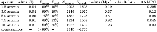
The galaxy counts are performed for 5 different radial aperture sizes: 1.5, 3, 5, 7.5, and 10 arcmin radius with no magnitude limit for the galaxies selected. Since an aperture size of about 0.5h50-1 Mpc in physical scale corresponding to about two core radii of a rich cluster provides a good sampling of the high signal-to-noise part of the galaxy overdensity in a cluster, the chosen set of apertures gives a good redshift coverage in the range from about z = 0.02 to 0.3 as shown by the values given in Table 4. With this choice and the depth limit of the COSMOS data set we are aiming at a high completeness in the cluster search out to a redshift of about z = 0.3. For this goal the chosen flux limit and the depth of the COSMOS data base are quite well matched as the richest and most massive clusters are still detected in both data sets out to this redshift.
The galaxy counts around the given
X-ray source positions are compared with the number count distributions
for 1000 random positions for each photographic plate.
With this comparison we are also accounting for plate to plate variations
in depth as explained below. The number count
histograms for the random positions have been generated at the
Naval Research Laboratory in preparation of a COSMOS galaxy cluster catalogue,
the SGP pilot study (Yentis et al. 1992; Cruddace et al. 2000), and for
this ESO key program. The results of the random
counts yield a differential probability density distribution,
![]() ,
of finding a number
of
,
of finding a number
of
![]() galaxies at random positions. An example for the distribution
galaxies at random positions. An example for the distribution
![]() for an average of 5 randomly selected plates is shown in
Fig. 9 for all five aperture sizes. (Note that
for an average of 5 randomly selected plates is shown in
Fig. 9 for all five aperture sizes. (Note that
![]() is defined here as a normalized probability density distribution
function while in Fig. 9 we show histograms of the form
is defined here as a normalized probability density distribution
function while in Fig. 9 we show histograms of the form
![]() ).
The distribution functions resemble
Poisson distributions (The possible theoretical description of the functions
is not further pursued here since we are only interested in the purely
empirical application to the following statistical analysis). In Fig. 10
the random count histogram for aperture 2 (3 arcmin radius) is
compared to the counting results for the 4206 X-ray source positions.
We note the large number of sources with significant galaxy
overdensities in the X-ray source sample compared to the random counts,
and expect to find the X-ray clusters in this high count tail
of the distribution.
).
The distribution functions resemble
Poisson distributions (The possible theoretical description of the functions
is not further pursued here since we are only interested in the purely
empirical application to the following statistical analysis). In Fig. 10
the random count histogram for aperture 2 (3 arcmin radius) is
compared to the counting results for the 4206 X-ray source positions.
We note the large number of sources with significant galaxy
overdensities in the X-ray source sample compared to the random counts,
and expect to find the X-ray clusters in this high count tail
of the distribution.
These results for
![]() are then used
in the form of cumulative probability distribution functions
are then used
in the form of cumulative probability distribution functions
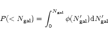 |
(1) |
Going back to the random sample, taking each of the values of
![]() assigned to each counting result, and plotting
the distribution function
assigned to each counting result, and plotting
the distribution function
![]() we will find that this function is a constant. This follows
simply from the chain rule of differentiation in the following
way
we will find that this function is a constant. This follows
simply from the chain rule of differentiation in the following
way
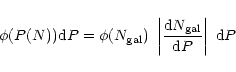 |
(2) |
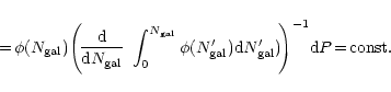 |
(3) |
For the further evaluation of this type of diagrams we make the following
simplifying assumptions: i) the distribution function is composed of
two types of counting results, results obtained for cluster
X-ray sources and results obtained for other sources, and ii) the
non-cluster X-ray sources are not correlated to the galaxy
distribution in the COSMOS data base and thus constitute effectively
a set of random counts. This latter assumption is of course not strictly
true for all the non-cluster X-ray sources. While it may be justified to
treat stars and other galactic sources as well as distant quasars
as independent of the nearby galaxy distribution, there is also a population
of extragalactic sources like low redshift AGN and starburst-galaxies
that we know are correlated to the
large-scale structure in the galaxy distribution.
However, the practical assumption that this correlation
is weak in comparison to the galaxy density enhancements in clusters of
galaxies is generally well justified.
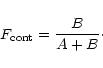
With this assumption we expect to find a distribution function
![]() composed of a constant function and a peak at
high P-values. Subtracting the constant function
leaves us with the cluster sources. This is
schematically illustrated in Fig. 12.
For the selection of the cluster candidates we can now either select
the sources which feature a high value of
composed of a constant function and a peak at
high P-values. Subtracting the constant function
leaves us with the cluster sources. This is
schematically illustrated in Fig. 12.
For the selection of the cluster candidates we can now either select
the sources which feature a high value of
![]() or a high
value of
or a high
value of
![]() .
We choose to use
.
We choose to use
![]() for the
sample selection (as justified further below) in such a way that most
of the cluster peak is included in the extracted sample (that is
choosing
for the
sample selection (as justified further below) in such a way that most
of the cluster peak is included in the extracted sample (that is
choosing
![]() such that the fraction C in Fig. 12
of cluster lost from the sample is small or negligible).
such that the fraction C in Fig. 12
of cluster lost from the sample is small or negligible).
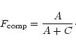 |
(4) |
 |
(5) |
 |
Copyright ESO 2001
![\begin{figure}
\par\includegraphics[width=8cm,clip]{aa10210f8.ps} %
\end{figure}](/articles/aa/full/2001/15/aa10210/img52.gif)
![\begin{figure}
\par\includegraphics[width=8cm,clip]{aa10210f9.ps}\end{figure}](/articles/aa/full/2001/15/aa10210/img62.gif)
![\begin{figure}
\par\includegraphics[width=7.8cm,clip]{aa10210f10.ps} %
\end{figure}](/articles/aa/full/2001/15/aa10210/img63.gif)
![\begin{figure}
\par\includegraphics[width=8cm,clip]{aa10210f11.ps} %
\end{figure}](/articles/aa/full/2001/15/aa10210/img70.gif)