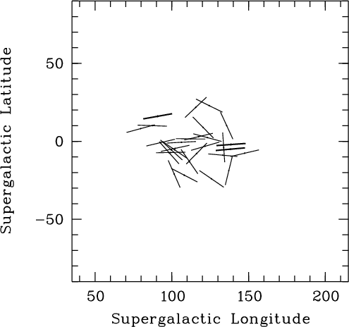
5%) do follow the
trend. This behavior is very reminiscent of the alignment of Galactic
star polarization vectors with the Galactic plane (Mathewson & Ford
1970; Axon & Ellis 1976).
5%) do follow the
trend. This behavior is very reminiscent of the alignment of Galactic
star polarization vectors with the Galactic plane (Mathewson & Ford
1970; Axon & Ellis 1976).
 and
and
 the latter constraint being
equivalent to
the latter constraint being
equivalent to
 ), or unpolarized (
 with
with
 ). The quasar type is also given: broad
absorption line (BAL), radio-loud non-BAL (RL), radio-quiet non-BAL
(RQ), or optically selected non-BAL (O). We may first notice that the
quasars with aligned polarization vectors do belong to all types, i.e.
radio-quiet/optically selected (3 objects), radio-loud (9), or BAL
(13). Note however that significantly polarized radio-quiet non-BAL
quasars are definitely less numerous, and that two of them,
B1115+080 and B1429-008, are possibly gravitationally
lensed. Furthermore, we can see that the known polarization difference
between BAL and non-BAL radio-quiet quasars also prevails in region A1
(Fig. 4). A Kolmogorov-Smirnov test gives a probability of only
0.6% that these two samples of are drawn from the same parent
population. The illustrated distributions are also in good agreement
with those reported by Hutsemékers et al. (1998). In addition, the
distribution of p for non-BAL radio-quiet quasars is very similar to
that found by Berriman et al. (1991) for the Palomar-Green quasar
sample. This clearly indicates that, also in region A1, quasar
polarization is related to the intrinsic properties of the objects.
). The quasar type is also given: broad
absorption line (BAL), radio-loud non-BAL (RL), radio-quiet non-BAL
(RQ), or optically selected non-BAL (O). We may first notice that the
quasars with aligned polarization vectors do belong to all types, i.e.
radio-quiet/optically selected (3 objects), radio-loud (9), or BAL
(13). Note however that significantly polarized radio-quiet non-BAL
quasars are definitely less numerous, and that two of them,
B1115+080 and B1429-008, are possibly gravitationally
lensed. Furthermore, we can see that the known polarization difference
between BAL and non-BAL radio-quiet quasars also prevails in region A1
(Fig. 4). A Kolmogorov-Smirnov test gives a probability of only
0.6% that these two samples of are drawn from the same parent
population. The illustrated distributions are also in good agreement
with those reported by Hutsemékers et al. (1998). In addition, the
distribution of p for non-BAL radio-quiet quasars is very similar to
that found by Berriman et al. (1991) for the Palomar-Green quasar
sample. This clearly indicates that, also in region A1, quasar
polarization is related to the intrinsic properties of the objects.
| Object | z | p |
 |
 |
 |
Ref | Type |
| (B1950) | (%) | (%) | (
 ) ) |
(
) |
|||
| B1115+080 | 1.722 | 0.68 | 0.27 | 46 | 12 | 0 | RQ |
| B1120+019 | 1.465 | 1.95 | 0.27 | 9 | 4 | 0 | BAL |
| B1127-145 | 1.187 | 1.26 | 0.44 | 23 | 10 | 2 | RL |
| B1138-014 | 1.270 | 0.38 | 0.23 | 53 | 21 | 9 | BAL |
| B1138+040 | 1.876 | 0.10 | 0.24 | 36 | - | 1 | RQ |
| B1157-239 | 2.100 | 1.33 | 0.17 | 95 | 4 | 9 | BAL |
| B1157+014 | 1.990 | 0.76 | 0.18 | 39 | 7 | 9 | RL |
| B1158+007 | 1.380 | 0.44 | 0.20 | 74 | 14 | 9 | RL |
| B1203+155 | 1.630 | 1.54 | 0.20 | 30 | 4 | 9 | BAL |
| B1205+146 | 1.640 | 0.83 | 0.18 | 161 | 6 | 9 | BAL |
| B1206+459 | 1.158 | 0.24 | 0.17 | 132 | 20 | 1 | RQ |
| B1210+197 | 1.240 | 0.33 | 0.19 | 76 | 19 | 9 | RL |
| B1212+147 | 1.621 | 1.45 | 0.30 | 24 | 6 | 0 | BAL |
| B1215+127 | 2.080 | 0.62 | 0.24 | 17 | 12 | 9 | BAL |
| B1216+110 | 1.620 | 0.58 | 0.19 | 63 | 10 | 9 | BAL |
| B1219+127 | 1.310 | 0.68 | 0.20 | 151 | 9 | 9 | BAL |
| B1222-016 | 2.040 | 0.80 | 0.22 | 119 | 8 | 9 | BAL |
| B1222+146 | 1.550 | 0.23 | 0.18 | 65 | 30 | 9 | O |
| B1222+228 | 2.046 | 0.84 | 0.24 | 150 | 8 | 2 | RL |
| B1225+317 | 2.200 | 0.16 | 0.24 | 150 | - | 2 | RL |
| B1228+122 | 1.410 | 0.12 | 0.18 | 142 | - | 9 | BAL |
| B1230-237 | 1.840 | 0.05 | 0.19 | 72 | - | 9 | O |
| B1230+170 | 1.420 | 0.30 | 0.19 | 101 | 22 | 9 | BAL |
| B1234-021 | 1.620 | 0.54 | 0.18 | 72 | 10 | 9 | O |
| B1235-182 | 2.190 | 1.02 | 0.18 | 171 | 5 | 9 | RL |
| B1238-097 | 2.090 | 0.18 | 0.18 | 80 | - | 9 | O |
| B1239+099 | 2.010 | 0.82 | 0.18 | 161 | 6 | 9 | BAL |
| B1239+145 | 1.950 | 0.18 | 0.20 | 21 | - | 9 | RQ |
| B1241+176 | 1.273 | 0.12 | 0.19 | 120 | - | 1 | RL |
| B1242+001 | 2.080 | 0.22 | 0.19 | 56 | 39 | 9 | RQ |
| B1246-057 | 2.236 | 1.96 | 0.18 | 149 | 3 | 8 | BAL |
| B1246+377 | 1.241 | 1.71 | 0.58 | 152 | 10 | 2 | RL |
| B1247+267 | 2.038 | 0.41 | 0.18 | 97 | 12 | 1 | RQ |
| B1248+401 | 1.030 | 0.20 | 0.19 | 3 | - | 1 | RQ |
| B1250+012 | 1.690 | 0.21 | 0.18 | 132 | 37 | 9 | BAL |
| B1254+047 | 1.024 | 1.22 | 0.15 | 165 | 3 | 1 | BAL |
| B1255-316 | 1.924 | 2.20 | 1.00 | 153 | 12 | 4 | RL |
| B1256-220 | 1.306 | 5.20 | 0.80 | 160 | 4 | 7 | RL |
| B1256-175 | 2.060 | 0.91 | 0.19 | 71 | 6 | 9 | RL |
| B1258-164 | 1.710 | 0.53 | 0.18 | 132 | 10 | 9 | O |
| B1303+308 | 1.770 | 1.12 | 0.56 | 170 | 14 | 3 | BAL |
| B1305+001 | 2.110 | 0.70 | 0.22 | 151 | 9 | 9 | O |
| B1309-216 | 1.491 | 12.30 | 0.90 | 160 | 2 | 4 | RL |
| B1309-056 | 2.212 | 0.78 | 0.28 | 179 | 11 | 0 | BAL |
| B1317+277 | 1.022 | 0.15 | 0.20 | 94 | - | 2 | RQ |
| B1329+412 | 1.930 | 0.36 | 0.21 | 83 | 16 | 1 | RQ |
| B1331-011 | 1.867 | 1.88 | 0.31 | 29 | 5 | 0 | BAL |
| B1333+286 | 1.910 | 5.88 | 0.20 | 161 | 1 | 9 | BAL |
| B1334+262 | 1.880 | 0.23 | 0.19 | 116 | 34 | 9 | BAL |
| B1338+416 | 1.219 | 0.37 | 0.19 | 67 | 15 | 1 | RQ |
| B1354-152 | 1.890 | 1.40 | 0.50 | 46 | 10 | 4 | RL |
| B1416+067 | 1.439 | 0.77 | 0.39 | 123 | 14 | 2 | RL |
| B1429-008 | 2.084 | 1.00 | 0.29 | 9 | 9 | 0 | RQ |
| B1429-006 | 1.180 | 0.07 | 0.20 | 107 | - | 9 | BAL |
| References: (0) Hutsemékers et al. 1998, (1) Berriman et al. | |||||||
| 1990, (2) Stockman et al. 1984, (3) Moore & Stockman 1984, | |||||||
| (4) Impey & Tapia 1990, (7) Visvanathan & Wills 1998, | |||||||
| (8) Schmidt & Hines 1999, (9) Lamy & Hutsemékers 2000. | |||||||
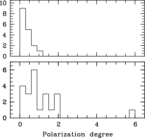 |
Figure 4: The distribution of the polarization degree p (in %) for the quasars located in the region of alignment A1 (Table 2). Upper panel: radio-quiet (RQ+O) quasars. Lower panel: BAL quasars |
 50 Mpc
scale, which is only slightly larger than the large-scale magnetic
field possibly detected by Vallée (1990) in the direction of the
Virgo cluster. But this interpretation suffers some drawbacks: namely,
it cannot explain why the polarization vectors of quasars at lower
redshifts are not accordingly aligned (cf. Fig. 5 in Paper I).
50 Mpc
scale, which is only slightly larger than the large-scale magnetic
field possibly detected by Vallée (1990) in the direction of the
Virgo cluster. But this interpretation suffers some drawbacks: namely,
it cannot explain why the polarization vectors of quasars at lower
redshifts are not accordingly aligned (cf. Fig. 5 in Paper I).
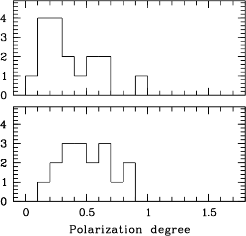 |
Figure 5:
The distribution of the polarization degree for the
radio-quiet (RQ+O) quasars in region A1. The upper panel is an
enlargement of that of Fig. 4 and refers to the observed polarization
degree p (in %). The so-called polarization bias (due to the fact
that p is always a positive quantity) affects the first bin (see also
Berriman et al. 1991). The lower panel shows the distribution of the
polarization degree after subtraction of a small but systematic
polarization (
 , ,
 ) )
|
 (for region A1), or all along the line of sight assuming a
cumulative or oscillatory effect (see also discussion in
Paper I). Interestingly, an oscillation of quasar polarization with
cosmological distance has been predicted as the consequence of the
conversion of photons into pseudo-scalars within a large-scale
magnetic field permeating the intergalactic medium (Harari & Sikivie
1992; Gnedin & Krasnikov 1992; Gnedin 1994). However, this
interpretation, like other mechanisms which affect light as it
propagates towards us, cannot easily explain why correlations observed
between quasar polarization and intrinsic properties are not washed
away.
In this view we may ask ourselves how small could be the systematic
polarization which, added to randomly oriented polarization vectors,
can be at the origin of an orientation effect which involves nearly
all polarized quasars of region A1. To simulate this, we have
vectorially subtracted a systematic polarization
(for region A1), or all along the line of sight assuming a
cumulative or oscillatory effect (see also discussion in
Paper I). Interestingly, an oscillation of quasar polarization with
cosmological distance has been predicted as the consequence of the
conversion of photons into pseudo-scalars within a large-scale
magnetic field permeating the intergalactic medium (Harari & Sikivie
1992; Gnedin & Krasnikov 1992; Gnedin 1994). However, this
interpretation, like other mechanisms which affect light as it
propagates towards us, cannot easily explain why correlations observed
between quasar polarization and intrinsic properties are not washed
away.
In this view we may ask ourselves how small could be the systematic
polarization which, added to randomly oriented polarization vectors,
can be at the origin of an orientation effect which involves nearly
all polarized quasars of region A1. To simulate this, we have
vectorially subtracted a systematic polarization  oriented at
(the dominant direction, cf. Fig. 1) from all
polarized and unpolarized quasars of region A1 (Table 2). Then
we have re-selected a sample of significantly polarized quasars with
the conditions
and
.
For
,
29 quasars fulfil the conditions
oriented at
(the dominant direction, cf. Fig. 1) from all
polarized and unpolarized quasars of region A1 (Table 2). Then
we have re-selected a sample of significantly polarized quasars with
the conditions
and
.
For
,
29 quasars fulfil the conditions![[*]](/icons/foot_motif.gif) and only 15
objects out of this new sample have their polarization position angles
still in the range
and only 15
objects out of this new sample have their polarization position angles
still in the range
 -
-
 .
This small systematic
polarization seems therefore sufficient to produce the orientation
effect, and small enough to preserve the difference between BAL and
non-BAL quasars. However, as seen in Fig. 5, even such a small
systematic polarization significantly modifies the polarization
distribution of non-BAL radio-quiet quasars which appears
depleted at polarization degrees
.
This small systematic
polarization seems therefore sufficient to produce the orientation
effect, and small enough to preserve the difference between BAL and
non-BAL quasars. However, as seen in Fig. 5, even such a small
systematic polarization significantly modifies the polarization
distribution of non-BAL radio-quiet quasars which appears
depleted at polarization degrees
 ,
and then quite
different from the distribution found by Berriman et al. (1991) and
Hutsemékers et al. (1998). If we further note that values of
higher than 0.25% are obviously needed to explain the alignment of
the 16 objects with
,
and then quite
different from the distribution found by Berriman et al. (1991) and
Hutsemékers et al. (1998). If we further note that values of
higher than 0.25% are obviously needed to explain the alignment of
the 16 objects with
 ,
we may conclude that it is quite
difficult to invoke a systematic additional polarization along the
line of sight without modifying the quasar intrinsic polarization
properties. This simple test also provides additional evidence that a
systematic instrumental effect is unlikely.
Although more subtle and speculative effects modifying the
polarization of light along the line of sight can probably be
imagined, we may admit on the other hand that the quasars themselves
i.e. their structural axes are coherently oriented on Gpc scales. For
radio-loud quasars, it is well known that the optical polarization is
often parallel to the structural axis of the radio core (Rusk 1990;
Impey et al. 1991). Unfortunately, only one polarized
quasar in region
A1 (B1127-145) is spatially resolved. It is however very interesting
to note that this object has a core structure parallel to its
polarization vector (Impey & Tapia 1990). In this view it is worth
noting that possible coherence of morphological structures from the
central engines of active galactic nuclei to superclusters has been
suggested by West (1991, 1994), although this observation is
apparently not confirmed at the supercluster scale (Jaaniste et
al. 1998). From the theoretical point of view, some studies (Reinhardt
1971; Wasserman 1978) have pointed out the possible effects of
magnetic fields on galaxy formation and orientation. Extrapolating, a
correlation between quasar structural axes could be settled at the
epoch of formation and related to very large-scale primordial magnetic
fields possibly formed during inflation (Battaner & Florido
2000). Large-scale vorticity is another possibility, at least
qualitatively. In this view, the apparent alignment found with the
supergalactic plane is puzzling. However, coincidence cannot be ruled
out, especially if we note that the polarization vectors of quasars
belonging to the other regions of alignments (regions A2 and A3 in
Paper I) do not show the same alignment with the plane of the Local
Supercluster.
,
we may conclude that it is quite
difficult to invoke a systematic additional polarization along the
line of sight without modifying the quasar intrinsic polarization
properties. This simple test also provides additional evidence that a
systematic instrumental effect is unlikely.
Although more subtle and speculative effects modifying the
polarization of light along the line of sight can probably be
imagined, we may admit on the other hand that the quasars themselves
i.e. their structural axes are coherently oriented on Gpc scales. For
radio-loud quasars, it is well known that the optical polarization is
often parallel to the structural axis of the radio core (Rusk 1990;
Impey et al. 1991). Unfortunately, only one polarized
quasar in region
A1 (B1127-145) is spatially resolved. It is however very interesting
to note that this object has a core structure parallel to its
polarization vector (Impey & Tapia 1990). In this view it is worth
noting that possible coherence of morphological structures from the
central engines of active galactic nuclei to superclusters has been
suggested by West (1991, 1994), although this observation is
apparently not confirmed at the supercluster scale (Jaaniste et
al. 1998). From the theoretical point of view, some studies (Reinhardt
1971; Wasserman 1978) have pointed out the possible effects of
magnetic fields on galaxy formation and orientation. Extrapolating, a
correlation between quasar structural axes could be settled at the
epoch of formation and related to very large-scale primordial magnetic
fields possibly formed during inflation (Battaner & Florido
2000). Large-scale vorticity is another possibility, at least
qualitatively. In this view, the apparent alignment found with the
supergalactic plane is puzzling. However, coincidence cannot be ruled
out, especially if we note that the polarization vectors of quasars
belonging to the other regions of alignments (regions A2 and A3 in
Paper I) do not show the same alignment with the plane of the Local
Supercluster.
Copyright ESO 2001