3 Observation and reduction

3.1 New spectroscopy

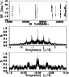
Figure 1: Spectroscopic observations of EN Lac. Top: time sampling. Center: window function. Bottom: window function zoomed at low frequencies

 

 

Table 2: Journal of observations. Authors (A) and instruments (I) are given below. $N_{\rm o}$, $N_{\rm r}$, and $N_{\rm l}$ list the number of observations, the number of runs, and the number of lines used for RV measurements. $w^{\rm w}$ and $w^{\rm s}$ are the calculated weights for the weak and for the strong weighting schemes, $RV_0^{\rm w}$ and $RV_0^{\rm s}$ are the corresponding finally calculated zero-point corrections

set	A	I	Epoch	$N_{\rm o}$	$N_{\rm r}$	$N_{\rm l}$	Disp.	$w^{\rm w}$	$w^{\rm s}$	$RV_0^{\rm w}$	$RV_0^{\rm s}$
			[JD-2400000]				[Åmm-1]			[kms-1]	[kms-1]
1	A	I	18542.7-24165.5	31	24	10-17	30	3.2	1.6	+3.3	+3.5
2	B	II	19631.8-21109.6	108	108	2-12	40	2.4	1.0	-2.0	-2.5
3	C	III	33869.7-33966.8	327	34	13	32	3.0	1.5	+0.6	+0.4
4	C	IV	33873.8-33877.0	47	4	13	10	7.0	3.4	-0.9	-1.4
5	C	V	33883.7-33925.9	68	43	7	11	6.7	2.7	-1.8	-1.8
6	D	V	34253.7-34984.9	36	20	5	11	6.7	2.3	-1.8	-1.8
7	D	VI	34258.6-34258.8	14	1	10	37	2.6	1.2
8	D	III	34909.8-34915.0	26	6	13	32	3.0	1.5	+0.6	+0.4
9	E	VII	40126.3-40128.4	19	3	23	76	1.0	0.5
10	F	VIII	43055.3-43058.6	51	4	23	12	6.4	3.2	+0.3	$\pm 0.0$
11	F	VIII	43417.3-43430.5	118	14	39	12	6.4	3.2	+0.3	$\pm 0.0$
12	G	IX	43459.7-44188.7	20	20	7	16.9	5.2	2.1
13	H	X	43738.0-43740.3	82	3	18	10	7.0	3.5	-0.6	-1.3
14	I	XI	45623.3-45631.5	47	9	41	9.65	7.1	3.5	-2.7	-2.6
15	J	XII	50279.4-51080.4	4	4	30	10	7.0	13.9	+0.9	+0.7
16	J	XIII	51009.5-51483.4	942	16	3	3.2	10.0	10.0	$\pm 0.0$	$\pm 0.0$
17	J	XIV	51436.7-51462.0	33	5	1	10	7.0	2.9	$\pm 0.0$	$\pm 0.0$
18	J	XV	48450.4-48457.6	205	5	40	8.1	7.7	15.2	+0.9	+0.7
19	J	XVI	48456.4-48456.6	45	1	40	5.2	8.9	17.7	+0.9	+0.7
20	J	XVII	50289.9-50294.0	7	4	1	10	7.0	2.9	$\pm 0.0$	$\pm 0.0$

Details on sources of data and instruments used. Column "A": A: Frost et al. (1926) (cf. also Lee 1910 and Struve & Bobrovnikoff 1925), B: Beardsley (1969), C: Struve et al. (1952), D: McNamara (1957), E: Bloch et al. (1970), F: LeContel et al. (1983), G: Abt et al. (1990), H: Sato & Hayasaka (1986) I: Chapellier et al. (1995), J: this paper. Column "I": I: Yerkes 1.02-m refractor, Bruce 1-prism spg., II: Allegheny 0.79-m Keeler Memorial reflector, 1-prism Mellon spg., III: Mt. Wilson 1.52-m reflector, Cassegrain spg., IV: Mt. Wilson 2.54-m reflector, coudé grating spg., V: Lick 0.91-m refractor, new Mills 3-prism spg., VI: Lick 0.30-m refractor, 2-prism spg., VII: Haute Provence 1.20-m reflector, prism spg., VIII: Haute Provence 1.52-m reflector, grating spg., IX: Kitt Peak National Observatory 1-m coudé feed grating spg., X: Okayama 1.88-m reflector, coudé grating spg., XI: Haute Provence 1.93-m reflector, grating spg., XII: this paper: Ondrejov 2.0-m reflector, coudé grating spg. with a Reticon RL 1872F/30 detector with 15 $\mu$m pixels, XIII: this paper: Tautenburg 2.0-m reflector, coudé echelle spectrograph with a Tektronix $1024\times1024$ CCD with 24 $\mu$m pixels, XIV: this paper: DAO 1.22-m reflector, coudé grating spg. with a thick Loral $4096\times200$ CCD with 15 $\mu$m pixels, XV, XVI: this paper: OHP 1.52-m reflector, Aurélie coudé grating spg. with a TH 7832 detector with 13 $\mu$m pixels, XVII: this paper: DAO 1.83-m reflector, Cassegrain grating spg.

Table 2 gives the journal of all RV observations at our disposal. Our own observations more than doubled the existing body of the data. Derived RVs are listed in Table 3. New spectra were obtained at four observatories:

1.

The dominant data set consists of 942 echelle spectra from the Thüringer Landessternwarte (TLS) Tautenburg. They were reduced with the help of MIDAS software by HL. The standard MIDAS software was modified for the wavelength calibration to obtain a perfect fit also at the overlapping edges of the echelle orders. RVs were obtained from the comparison of the synthetic and observed line profiles for the three cleanest (least blended) He I lines: 5015, 5875, and 6678 Å;

2.

The second largest set is a series of blue (4400-4700 Å) and green (4750-5050 Å) Aurelie spectra secured with the 1.52-m reflector of the Haute Provence Observatory (OHP) during 8 consecutive nights. Their initial reduction (bias subtraction, flat-fielding) was done by PM. The wavelength calibration and RV measurements were carried out by PH who used the SPEFO program - see Horn et al. (1996) and Skoda (1996). RVs of symmetric and stronger metallic lines (mostly O II, N II and C II), H$\beta$ and He I 4472 and 4923 Å lines were measured. Their wavelengths were derived from measurements of synthetic spectra broadened to the projected rotational velocity of EN Lac. Only lines which were symmetric in the synthetic spectra were used;

3.

Four red (6280-6720 Å) Reticon spectra were obtained in the coudé focus of the Ondrejov 2.0-m reflector. They were completely reduced with SPEFO by PH. RVs were derived from He I 6678 Å, H$\alpha$and several stronger and symmetric metallic lines;

4.

Several red (6100-6750 Å) CCD spectrograms were obtained at the Dominion Astrophysical Observatory (DAO). They were completely reduced within IRAF and MIDAS by SY and DH. Only RV of the He I 6678 Å line was measured.

For all spectra covering the red wavelength region the instrumental RV zero-points were derived with the help of a large set of telluric O₂ and H₂O lines. This allows us to assume that the above datasets 1, 3 and 4 (sets 15, 16, 17 and 20 of Table 2) are on exactly the same heliocentric wavelength scale. Note that due to the fitting procedures all RVs correspond to the RVs of line centroids and not of line minima.

3.2 Data from literature

We compiled all series of RV observations available in the astronomical literature and used a computer program to derive heliocentric Julian dates (HJDs hereafter) from the tabulated dates of mid-exposures or geocentric Julian dates for all of them. This way we found a few misprints in tabulated JDs for RVs of EN Lac published by Beardsley (1969). For convenience of future investigators, they are summarized in Table 4. For JD 2420038 it is not clear whether the misprint occurred for the date or the Julian date and we omitted this observation from our data set. Figure 1 shows the sampling of all RVs in time and also the window function of the data which will be discussed later.

 

 

Table 4: Misprints detected in tabulated times of observations of EN Lac in Beardsley (1969)

Date (G.M.T.)	Tabulated JD	Correct JD
	-2400000	-2400000
1913 Sep. 27.621	20038.671	?
1914 Sep. 22.746	20389.746	20398.746
1916 Sep. 02.631	21107.631	21109.631

3.3 Weighting scheme

Our compilation of RVs is very inhomogeneous. Spectra were observed with different instruments and have very different linear dispersions and resolutions. Also RVs were derived by different authors and rest on different sets of spectral lines. A part of them comes from photographic plates and another one from electronic spectra. So we have a set of RVs of different accuracy and probably also of a slightly different zero point of the RVscale.

To take these differences at least partly into account, we attempted to find out a suitable weighting scheme. This is not simple in our particular case. Due to steady improvements of the observational and reduction techniques, the accuracy, and therefore the weights would, on average, increase with time. We have recent observations of a high accuracy, well suited for precise RV measurements. However, the older, less accurate observations are invaluable to a search for the long-term amplitude changes over the periods of years or even decades.

The trouble is that any weighting scheme with a steep dependence on, say, the dispersion of the spectra (a strong weighting hereafter) almost completely suppresses the older observations. Consequently, we used three different weighting schemes: unweighted data, weak weighting, and strong weighting. Unweighted data will be used to derive a complete multiple-frequency fit and to include long-term amplitude modulation of rapid oscillations. Weighted data will be used to verify and improve the frequencies found in the first step and to derive an accurate orbital solution.

Strong weighting: The error of a RV value derived from a single spectral line profile I(RV)follows from the photon statistics (Butler et al. 1996):

$$\sigma^{-2}_i = \sum{\left(\frac{{\rm d}I(RV)}{{\rm d}RV}\right)^2\,N_{\rm ph}(RV)}.$$ (1)

The accuracy of a RV measurement at a certain point of the line profile is determined by the local gradient of the profile and the number of photons $N_{\rm ph}$ collected at this point. The sum extends over all discrete measurements (steps in RV) taken to derive the RV of line i. Assuming a Gaussian line profile and a small central line depth A_i, it follows that

$$\sigma_i \propto A^{-1}_i f(D),$$ (2)

where f is a function of the dispersion, but also of $v\sin(i)$ and of the resolution of measurement limited by the projected slit width of the spectrograph, or possibly by the pixel size of the electronic detector or the point spread function of the photographic plates. Petrie (1962) tabulated the mean RV errors found from single-line measurements in photographic spectra of various dispersions. A least squares fit to his values for B-type stars give

$$f(D) \propto 1.33 + 0.042\,D,$$ (3)

where D is in Åmm^-1 and f is in kms^-1. If the mean RV, based on measurements of N lines, is computed from unweighted data, as we will assume here, the error of the mean follows as

$$\sigma^2 \propto f^2 N^{-2} \sum A^{-2}_i.$$ (4)

To estimate the sum in Eq. (4) we will assume that in any spectrum the Nstrongest lines were used. In that case the sum can be estimated from the inverse frequency distribution of line depths in the spectrum. For EN Lac we obtain from an analysis of the TLS spectra an approximate distribution of $A^{-1}_i \propto 0.9+0.1\,i$, where i=1 stands for the strongest metal line (the 11th strongest line of the spectrum has a line depth of about half of the depth of the strongest line).

The weight w of a RV value should be $w \propto \sigma^{-2}$ which leads to the final formula

$$w = \frac{Q\,N^2}{(1.33+0.042\,D)^2 \sum(0.9+0.1\,i)^2}\cdot$$ (5)

The summation goes over the N lines measured in a given spectrum. The superior S/N ratio of the electronic spectra is taken into account via an additional multiplicative factor Q. We set Q=1 for photographic and Q=4 for electronic spectra.

Since we assumed that unweighted mean RVs are derived by most of the authors, the approximately assumed steadily decrease of line depth with increasing N results in a maximum of the weights for $N \sim 16$. We, therefore, set in Eq. (3) N=16for all RVs derived from more than 16 lines.

Weak weighting: To test the influence of weighting on the obtained results we also used a weak weighting for a comparison. We assumed that the accuracy of RVs depends only on the linear dispersions and use Eq. (3) to calculate the weights, with $w\sim f^{-2}$. The adopted weights for the individual data sets and for both weighting schemes are also given in Table 2. Weights were normalized in such a way that w=10 for the TLS data.

The question of different instrumental RV zero-points will be discussed later in connection with the multiple period search.