4 Disentangling orbital and short-term $\vec {RV}$ changes

4.1 Period finding techniques

Three different computer programs were used to calculate the orbital solution and to search for, and model the short-period changes. The first program derives the orbital solution by the method of differential corrections to the initial orbital elements (Schlesinger 1908; Sterne 1941). The program optimizes the orbital elements including the orbital period. It can handle data with unequal weights, and it is possible to include the apsidal advance among the elements.

The second program uses a multiple period finding technique which is able to optimize arbitrary frequencies and its harmonics. It is based on a least-squares fit of sinusoids. For very low eccentricities, as in the case of EN Lac, the program fits the orbital curve very well using only the fundamental period and its first harmonic. It is, therefore, possible to obtain a simultaneous fit of orbital as well as pulsational periods at one iterative process. All but one of the periods are fixed. To optimize the whole family of frequencies involved, the procedure is iteratively repeated for individual frequencies. In a sense, the program represents an extension of the well-known CLEAN algorithm since not only one single period but also the amplitudes and phases of all included periods are optimized.

The third program computes a modified Scargle periodogram the ordinate of which corresponds to the reduction of the sum of squares by the least squares fit of sinusoids used. A detailed description of the periodogram and a discussion of its statistical properties can be found in Lehmann et al. (1999). The program is used to search in the residuals of an assumed multiple frequency model for possible additional frequencies.

Some principal results were also independently verified with the help of program FOTEL - see Hadrava (1990).

4.2 Orbital solution for the original RVs

When the oscillations show constructive interference, the amplitude of the observed short-term RV variations is nearly comparable to the semi-amplitude of the orbital RV curve. This complicates the determination of truly reliable orbital elements. One can of course make use of the fact that the three periods of oscillations, P₁ = 0 $.\!\!^{\rm d}$1691678, P₂ = 0 $.\!\!^{\rm d}$1707769, and P₃ = 0 $.\!\!^{\rm d}$1817331, have been well established from photometric observations. However, the amplitudes of these oscillations are known to vary with time which represents an extra complication for the frequency analysis.

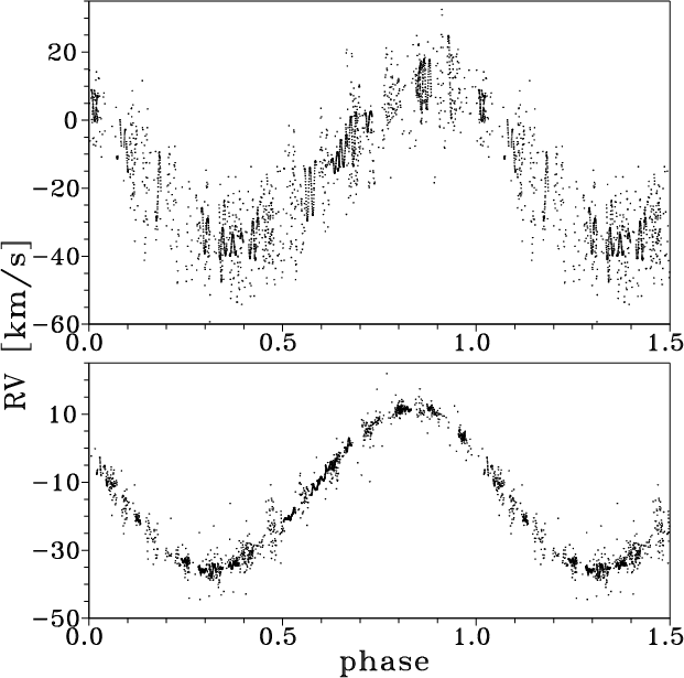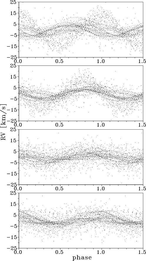
Figure 2: Top: orbital solution I derived from raw data. Bottom: orbital solution II derived from the same data but prewhitened for the short-term variations found in selected data groups

 

 

Table 5: Orbital elements. Epochs are in JD - 2400000

	Solution I			Solution II
P [d]	12.096860	$\pm$	0.000026	12.096844	$\pm$	0.000010
K [kms-1]	23.66	$\pm$	0.18	23.818	$\pm$	0.033
$\gamma$ [kms-1]	-12.52	$\pm$	0.13	-12.289	$\pm$	0.026
e	0.0347	$\pm$	0.0090	0.0392	$\pm$	0.0017
$\omega$ [deg]	65	$\pm$	12	63.7	$\pm$	2.1
$T_{\rm periastron}$	39053.77	$\pm$	0.41	39053.71	$\pm$	0.07
$T_{\rm eclipse}$	39054.55	$\pm$	0.78	39054.53	$\pm$	0.14
rms	6.03 kms-1			1.10 kms-1

 

 

Table 6: Periods found within the data groups. Sets are as in Table 2, $N_{\rm s}$ is the total number of spectra, $N_{\rm r}$ the number of runs. P and K give the periods in days and semi-amplitudes in kms^-1, respectively. P₁ to P₃ refer to periods near to the known triplet of short-term variations, all other periods are listed as P₄

group	set	mean JD	$N_{\rm s}$	$N_{\rm r}$	P1	K1	P2	K2	P3	K3	P4	K4
1	2	19699.6	39	39	.16918	8.6	.17078	3.0	.18165	2.4
2	2	20054.0	52	52	.16920	7.9	.17092	3.4	.18169	5.6
3	3	33923.4	327	15	.16915	15.5	.17070	2.9	.18179	1.6
4	4	33874.9	47	4	.16865	11.7					1.733	1.9
5	5	33904.9	68	7	.16917	13.7	.17081	4.5	.18106	1.0
6	6	34795.8	36	4	.16924	15.1	.17078	4.1	.18173	4.2
7	8	34913.0	26	2	.16961	18.9
8	10	43057.3	51	4					.18193	4.5	.16961	7.4
9	11	43425.0	118	7	.16931	5.2	.17076	1.9	.18173	2.6
10	13	43739.3	82	3	.16831	7.5			.18073	4.8	.2896	2.1
11	14	45627.6	47	5	.16916	4.2	.17348	1.0	.18166	5.2
12	18+19	48453.8	250	6			.16986	5.7	.18179	6.4	.19701	1.1
13	16	51110.4	229	6	.16917	1.9	.17323	4.4			.19545	2.2
14	16	51437.1	714	9	.16917	3.9	.17083	3.1	.18171	2.0	.17258	2.0
15	17	51449.5	33	4	.16921	3.7	.17084	4.0	.18193	0.8

To disentangle the orbital motion and short-term RV changes, we proceeded in two different ways. In the first step, we derived an initial solution (solution I of Table 5) using all the original RVs of Table 2 and adopting the weak weighting. This is why the scatter around the mean orbital RV curve displayed in the upper panel of Fig. 2 looks larger than the calculated mean rms per one observation: the scatter is mainly caused by low-dispersion data with small weights. A small part of the scatter is also due to the fact that we assumed one joint systemic velocity for all RVs at this stage.

4.3 Investigation of data subsets

To proceed further, we created subsets of RV data, spanning not more than 180 d. Moreover, each subset was formed in such a way that it contains data from only one source and from one spectrograph and also enough RVs with a sufficient sampling in time to allow a separate period search for rapid changes. This way, we formed 15 different subsets which are listed in Table 6. Then we subjected the O-C velocity residuals from solution I for each of the subsets to a period search in the neighbourhood of the known periods P₁ to P₃. Using a least-squares sinusoidal fit of these three periods within each subset, we prewhitened the original RVs for the rapid changes. Prewhitened RVs from all subsets were then combined and used to calculate a new orbital solution. The process was iterated until convergence was achieved. The final orbital solution is given as solution II in Table 5. No evidence of apsidal motion was found. It is seen that the decrease of the mean rms error per 1 observation between solutions I and II is quite substantial.

Figure 3: A plot of the semi-amplitude of the P1-variation of Table 6 vs. time. The solid curve is a sinusoid with a period of 23000 d

Table 6 shows that for a few subsets, we arrived at rather peculiar values of the short periods. In some cases, only one or two periods are detectable. A significant result of our analysis is the finding that the amplitude of P₁ varies with an apparent cycle of about 23000 d - see Fig. 3. Possible time scales for the amplitude variation of P₃ are 237, 473 or 673 d, the latter value being reported already by Jerzykiewicz & Pigulski (1996) from their analysis of photometric data. There is no evidence of a periodic modulation of the amplitude of P₂.

4.4 Properties of the triplet of short periods

Note that our approach differs from that used by Jerzykiewicz & Pigulski (1996) who fixed the values of the three short periods at their values known from photometry and fitted only their amplitudes. They concluded that the amplitudes are strongly variable with time. For completeness, we repeated their analysis using all our RVs prewhitened for orbital variation via solution II. The results are compared in Table 7. It is seen that a free fit of the periods leads to much larger semiamplitudes for all three considered periods than a fit with fixed values of the periods from photometry. Moreover, the phase diagram of the data prewhitened for P₂ and P₃ and folded with P₁ shows a clear phase shift between the older, more scattered RVs of higher amplitude and the CCD data with a lower amplitude - see the upper panel in Fig. 4.

If one allows for a free convergence of all three periods, it is possible to arrive at somewhat larger amplitudes and a better phase coherence for P₁. There are remaining phase shifts, however, especially for P₂ and P₃, and it is clear that the three known frequencies are unable to model the large amplitudes of P₁ (up to 18 kms^-1 during certain epochs) properly. For P₂ we arrived at a one-year alias of the reported photometric period. This value was also found by others, as already mentioned in Sect. 2.

 

 

Table 7: Periods and semi-amplitudes of the short-term triplet found in the data prewhitened for orbital solution II

periods fixed		periods optimized
P [d]	K [kms-1]	P [d]	K [kms-1]
.1691678	3.8	.16916714	5.7
.1707769	0.9	.17085757	2.6
.1817331	2.1	.18171870	2.7

Figure 4: Phase diagrams folded with the periods of P1 to P3 of the data prewhitened for the orbital and the corresponding two other short-term distributions. From top to bottom: P1, all short-term periods fixed to the values from photometry, P1 from optimized short-term periods, P2 optimized, P3 optimized

4.5 A free search for multiperiodicity

At this stage of investigation it is legitimate to ask whether a free search for multiperiodicity, not necessarily restricted to the three known periods, can significantly improve the fit of the RV residuals from the orbit and offer a self-consistent solution, at least comparable to our locally fitted solution presented in Sect. 4.3.

The varying accuracy of the RVs was taken into account through the weighting schemes already described. To check on possible differences in the RVzero-points of individual data sets, we will now include only data sets with large enough RVs, with a good orbital-phase coverage. Applying these requirements, we finally selected all data sets from Table 2 with the exception of subsets 7, 9, and 12. We may assume that the RV zero-point of our own measurements, calibrated via telluric lines (data sets 15, 16, and 17) is identical and equal to zero in the RV residuals. We will further assume that the subsets 3 and 8 have a common zero point, similarly as subsets 5, 6, 3, and 8, 10, 11, and 18, 19. All these groups were obtained with the same instruments and have comparable weights.

We started with prewhitening the selected set of RVs, formed by all of above-mentioned subsets, for orbital solution II. The RV residuals from this prewhitening were then subjected to a period search over the frequency range from 0 to 10 d^-1. The frequency corresponding to the strongest peak in the periodogram was then improved via sinusoidal fit and removed from the data. The new residuals were again subjected to a period search and the sinusoidal fit was repeated, now for two free periods. After finding three short periods near to the photometric periods P₁ to P₃, a multiperiodic fit was applied to the original RVs and allowed to calculate also the orbital frequency and its first harmonics. (Note that this procedure is legitimate as long as there is no detectable apsidal motion present in the system.)

Since the results could be sensitive to possible differences in the RV zero points, parallel analyses were carried out for original data and for data where the zero-point corrections were taken into account. To compute the zero-point corrections the residuals from the multiperiodic fit were averaged within each data subset and the mean value was subtracted from all RVs of the subset in question. As long as the same new frequency was found in both parallel analyses, it was adopted as a real one, i.e. not caused by differing RVzero-points only.

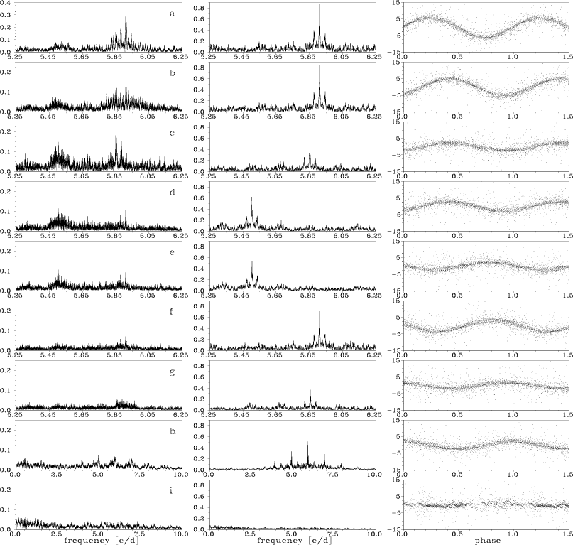Figure 5: Left column: periodograms obtained during the process of successive prewhitening. The following detected periods of Table 9 are indicated: a) P1, b) P1-, c) P2, d) P3, e) P3+, f) P1+, g) P2+, h) P1++, i) P4. Middle and right column: periodograms and phase diagrams for the same periods are also shown, based on the final solution, after the RVs were prewhitened for all other contributions

 

 

Table 8: Multiple frequency solution valid for all weighting schemes used. Periods P and their semi-amplitudes K are given. Column "Order" gives the order in which the periods were found during the process while $t_{\rm amp}$ contains the probable periods of amplitude changes of the respective periods

	Order	P	K	$t_{\rm amp}$
		[d]	[kms-1]
P1	1	0.16916707	7.6
P1+	4	0.16916605	5.0	76.7 y
P1-	2	0.16916809	3.2	76.7 y
P2	7	0.17085553	2.7
P2+	3	0.17077074	1.4	344 d
P3	5	0.18173251	2.6
P3+	6	0.18168352	2.4	674 d

 

 

Table 9: Periods P and semi-amplitudes K, including the period P₁⁺⁺, which could only be detected in data with strong weighting. P₄ is not a significant period but the period corresponding to the largest peak in the residuals. Otherwise, the same notation as in Table 8 was used

	Order	P	K	$t_{\rm amp}$
		[d]	[kms-1]
P1	1	0.16916703	5.9
P1+	4	0.16916596	5.2	73.6 y
P1-	2	0.16916810	3.5	73.6 y
P1++	8	0.16916078	2.3	12.5 y
P2	7	0.17085554	2.2	331 d
P2+	3	0.17076729	1.6
P3	5	0.18173256	2.8	674 d
P3+	6	0.18168357	2.3
P4	9	1.91985	0.7

The obtained results are summarized in Tables 8 and 9. The periods which were detected in our analyses and which are very close to the three known photometric periods are denoted here as P₁, P₂and P₃. Newly found periods, which are very close to P₁, P₂ or P₃and which can be responsible for the amplitude modulation of the periods P₁, P₂ and P₃, are denoted $P_i^\pm$ in such a way that

$$f_i^\pm = f_i\pm {\rm d}f_i,$$ (6)

where f_i are the corresponding frequencies for i = 1, 2, 3and $({\rm d}f_i)^{-1}$ is a period corresponding to the amplitude variation of the respective principal period.

We stopped at the point when different new frequencies were detected from different weighting schemes. Table 8 summarizes the results for this stage of reduction. Beside the values of P₁ to P₃, two "sidelobes'' of P₁, responsible for the amplitude modulation of P₁ with a period of 76.7 years, and two frequencies very close to P₂ and P₃ and corresponding to their amplitude modulation with 344-d and 674-d periods, respectively, were detected.

 

 

Table 10: Final orbital solutions III (corresponding to Table 8) and IV (Table 9) after subtracting all short term contributions. Epochs are in JD-2240000

	Solution III			Solution IV
P [d]	12.096867	$\pm$	0.000010	12.096864	$\pm$	0.000011
K [kms-1]	23.858	$\pm$	0.051	23.853	$\pm$	0.051
$\gamma$ [kms-1]	-12.694	$\pm$	0.039	-12.446	$\pm$	0.039
e	0.0435	$\pm$	0.0026	0.0539	$\pm$	0.0026
$\omega$ [deg]	59.4	$\pm$	2.9	61.4	$\pm$	2.1
$T_{\rm periastron}$	39053.59	$\pm$	0.10	39053.65	$\pm$	0.10
$T_{\rm eclipse}$	39054.54	$\pm$	0.20	39054.52	$\pm$	0.17
rms	1.7 kms-1			1.5 kms-1

Figure 6: Final orbital solution IV after subtracting all short-term contributions

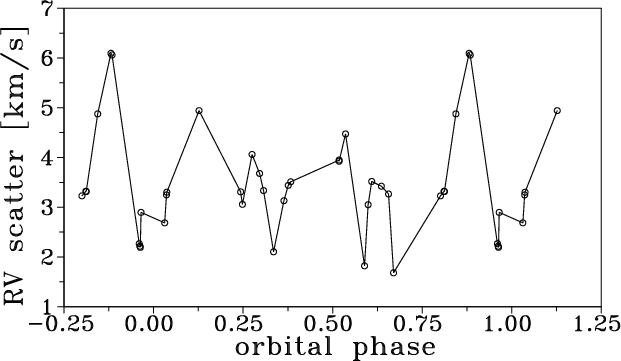Figure 7: The RV phase scatter vs. orbital phase with phase zero at periastron passage - see the text for details

No other periods could be detected in the residuals from this solution for the unweighted data. In the weakly weighted data, the strongest peak suggests yet another period of 0 $.\!\!^{\rm d}$202, which, however, does not seem to be significant (semi-amplitude of 0.4 kms^-1 and a very unconvincing phase diagram). From the strongly weighted data, another period very close to P₁ was indicated. A free fit for all detected periods changes the period of the amplitude modulation of P₂ from 344 d to 331 d, however. The solution derived from the strongly weighted data is summarized in Table 9 and the successive periodograms are shown in Fig. 5. Middle panels show the periodograms for each of the periods resulting after subtraction of all other contributions obtained in the final solution. Comparing panels a to g of this column (panels h and i are on enlarged frequency scale) one can recognize the window function of the data shown in Fig. 1. The one-month aliases can clearly be seen. In all periodograms also the one-year alias peaks can be found (not resolved in Fig. 1). Note that the difference of the two frequencies found for the P₂ variation corresponds to 331 d so that the two frequencies are not one-year aliases of each other. In the right column of Fig. 5 the phase diagrams of each period, after prewhitening the data for all other periods, are shown.

The orbital solutions, based on RVs prewhitened for all short periods of Tables 8 and 9, are presented in Table 10 as solutions III and IV, respectively. For comparison we also give the calculated epochs of primary mid-eclipse. Pigulski & Jerzykiewicz (1988) derived $P = 12\hbox{$.\!\!^{\rm d}$ }09684$ and $T_{\rm eclipse} = 39054.568$ from the light-curve analysis. Note that the epoch of the primary mid-eclipse from all of our orbital solutions agrees with their epoch within the errors of its determination. A phase diagram corresponding to solution IV is shown in Fig. 6.

Solutions III and IV are based on RVs corrected for the zero-point shifts and on strong weights. The results are almost identical to those derived without the zero-point corrections. In particular, there is only a marginal difference of 0 $.\!\!^{\rm d}$000007 in the orbital period. The adopted zero-point corrections are summarized in Table 2.

4.6 Search for signatures of forced oscillations

To demonstrate that the rapid variations of EN Lac are somehow related to the binary nature of the star is not an easy task, especially given the fact that the amplitude of the strongest mode of oscillations varies secularly. Fortunately, the rich collection of new spectra analyzed here was obtained over a limited period of time and seems suitable to such an analysis.

Using all 1315 original RVs from spectrograms of sets 16 to 20, we formed phase bins 0.$^{\rm P}$07 wide in three sliding representations - similar to three different "covers'' in the phase dispersion minimization method of Stellingwerf (1978). (The width of the bins was chosen in such a way as to ensure numerous enough representation in most of them.) We then calculated mean RV and its rms error within each such phase bin. The rms error characterizes the total scatter at given orbital phase and should be proportional to the total amplitude of rapid changes at that phase. Omitting all bins defined by less than 30 RVs, we plot the phase scatter versus orbital phase calculated from periastron in Fig. 7. There seems to be a rapid increase of the scatter prior and perhaps also after each periastron passage, though the effect is only marginal. Still more data will be needed to verify that it is a real effect dependent on orbital phase and not, e.g., an accidental effect of positive interference of several pulsational modes.