| Issue |
A&A
Volume 578, June 2015
|
|
|---|---|---|
| Article Number | A55 | |
| Number of page(s) | 24 | |
| Section | Interstellar and circumstellar matter | |
| DOI | https://doi.org/10.1051/0004-6361/201424364 | |
| Published online | 04 June 2015 | |
Online material
Appendix A: On the late-time ortho/para ratios of ammonia and water
In the ISM, ammonia production is dominated by the electron recombination of the ammonium ion, ![]() , and its destruction occurs mainly through a charge transfer reaction with H+. At late times of chemical evolution, the proton transfer reaction with
, and its destruction occurs mainly through a charge transfer reaction with H+. At late times of chemical evolution, the proton transfer reaction with ![]() returns ammonia back to
returns ammonia back to ![]() . The dominant reactions are shown schematically in Fig. A.1. The destruction rates of pNH3 and oNH3 in reactions with H+,
. The dominant reactions are shown schematically in Fig. A.1. The destruction rates of pNH3 and oNH3 in reactions with H+, ![]() , and
, and ![]() are equal, and consequently the o/p-NH3 ratio is determined by the nuclear spin branching ratios in the electron recombinations of para-, ortho-, and meta-
are equal, and consequently the o/p-NH3 ratio is determined by the nuclear spin branching ratios in the electron recombinations of para-, ortho-, and meta-![]() . One obtains the relationship
. One obtains the relationship  (A.1)The ammonium ion is predominantly formed in the reactions
 ![]() and
and ![]() . These reactions determine the nuclear spin ratios of
. These reactions determine the nuclear spin ratios of ![]() , because the electron recombination rates are equal for the different nuclear spin species. The following relationships are obtained:
, because the electron recombination rates are equal for the different nuclear spin species. The following relationships are obtained:  (A.2)The primary production pathway to
 ![]() ,
, ![]() , becomes at late times less important than the charge transfer reaction between NH3 and H+, and in this situation one obtains roughly equal o/p ratios for NH3 and
, becomes at late times less important than the charge transfer reaction between NH3 and H+, and in this situation one obtains roughly equal o/p ratios for NH3 and ![]() :
: ![]() (A.3)Finally, substituting Eqs. (A.2) and (A.3) to Eq. (A.1), one obtains (with a little algebra) the steady-state ratio
(A.3)Finally, substituting Eqs. (A.2) and (A.3) to Eq. (A.1), one obtains (with a little algebra) the steady-state ratio ![]() (A.4)This value is about 10% lower than the one predicted by our simulation with the full reaction set.
(A.4)This value is about 10% lower than the one predicted by our simulation with the full reaction set.
The ammonia abundance in interstellar molecular clouds is frequently derived using observations of the (1, 1) and (2, 2) inversion lines at λ = 1.2 cm, which both represent para-NH3. The total ammonia abundance is then derived by assuming o/p − NH3 = 1 or that the ortho and para states are populated according to LTE. The latter assumption implies at 10 K that o/p − NH3 = 3.3. Our result suggests that these previous observational estimates of the total ammonia abundance can be unrealistically large.
 |
Fig. A.1
Ammonia cycle at late times of chemical evolution. |
| Open with DEXTER | |
Water is produced primarily in the electron recombination of the hydronium ion, H3O+ and, like ammonia, destroyed mainly in the charge transfer reaction with H+. The recombination of pH3O+ yields both oH2O and pH2O at equal ratios, whereas oH3O+ only yields ortho-water (along with hydroxyl). We obtain the relationship ![]() (A.5)
(A.5)
The H3O+ production is dominated by H2O+ + H2 → H3O+ + H. The spin selection rules result in the relationship  (A.6)
(A.6)
 |
Fig. A.2
Dominant reactions involving water and hydroxyl. |
| Open with DEXTER | |
The most important reactions determining the abundance of water and related molecules in the gas phase are shown in Fig. A.2. The dominant pathway to H2O+ is the H atom abstraction reaction OH+ + pH2 → (poro)H2O+ + H, which leads to pH2O+ and oH2O+ with equal probability. The second reaction of importance is the charge transfer reaction H2O + H+ (with a 20% share of the H2O+ production), and the third is proton transfer from ![]() (~10%). Omitting the secondary reactions, one obtains
(~10%). Omitting the secondary reactions, one obtains ![]() (A.7)The full reaction set yields o/p − H2O+ ~ 1.6 at late times. The substitution of Eqs. (A.6) and (A.7) to Eq. (A.5) yields a value
(A.7)The full reaction set yields o/p − H2O+ ~ 1.6 at late times. The substitution of Eqs. (A.6) and (A.7) to Eq. (A.5) yields a value ![]() (A.8)representing steady state. This is about 20% lower than the late-time o/p ratio in our simulation. This discrepancy can be understood by the fact that in the very simple model described above, we have omitted the production of H2O+ from H2O and OH.
(A.8)representing steady state. This is about 20% lower than the late-time o/p ratio in our simulation. This discrepancy can be understood by the fact that in the very simple model described above, we have omitted the production of H2O+ from H2O and OH.
Appendix B: New branching ratios for water chemistry and updates to S13
Branching ratios of the most important reactions in the water formation network.
Rate coefficient data from Le Gal et al. (2014) included in the present model.
Appendix C: Calculations at different temperatures
In this appendix, we present the results of calculations otherwise similar to those presented in Sect. 3, but produced assuming either Tgas = Tdust = 15 K or Tgas = Tdust = 20 K.
 |
Fig. C.1
As for Fig. 2, but calculated with Tgas = Tdust = 15 K. |
| Open with DEXTER | |
 |
Fig. C.2
As for Fig. 3, but calculated with Tgas = Tdust = 15 K. |
| Open with DEXTER | |
 |
Fig. C.3
As for Fig. 4, but calculated with Tgas = Tdust = 15 K. |
| Open with DEXTER | |
 |
Fig. C.4
As for Fig. 2, but calculated with Tgas = Tdust = 20 K. |
| Open with DEXTER | |
 |
Fig. C.5
As for Fig. 3, but calculated with Tgas = Tdust = 20 K. |
| Open with DEXTER | |
 |
Fig. C.6
As for Fig. 4, but calculated with Tgas = Tdust = 20 K. |
| Open with DEXTER | |
Appendix D: Calculations without deuterium
Including deuterium in a chemical model may decrease the abundances of nondeuterated species especially at high densities in the presence of depletion, where deuterium fractionation is strong. To investigate how our results change when deuterium is excluded, we ran model calculations at T = 10 K setting the initial HD abundance (i.e., the initial deuterium abundance) to zero. The results of these calculations are presented in Figs. D.1 to D.3, which should be compared against Figs. 2 to 4 in the main text.
It is observed that in the gas-phase model, where there is little deuteration regardless of density, excluding deuterium from
the calculations makes virtually no difference in the abundances of the non-deuterated species. Even in the gas-grain model, only very small enhancements are observed in the abundances of non-deuterated species at high density. Also, the o/p ratios of H2O and NH3 are only very slightly modified in the gas-grain model, and hardly at all in the gas-phase model. Our models thus imply that disregarding deuteration in chemical models when T ≳ 10 K will likely not lead to large errors in the abundances of non-deuterated species. We note that we have not carried out a full parameter-space exploration of this issue here, and have only explored the effect of density (and temperature; Appendix C) on the results.
|
Fig. D.1
Abundances of selected species in a gas-phase model excluding deuterium. This figure should be compared to Fig. 2. |
|
| Open with DEXTER | |
|
Fig. D.2
Abundances of selected species in a gas-grain model excluding deuterium. This figure should be compared to Fig. 3. |
|
| Open with DEXTER | |
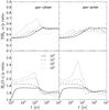 |
Fig. D.3
As for Fig. 4, but excluding deuterium. |
| Open with DEXTER | |
Appendix E: Calculations with quantum tunneling included
Below, we present the results of calculations performed at T = 10 K, but including quantum tunneling on grain surfaces. When tunneling is included, the thermal diffusion rate defined by Eq. (9) is replaced by the tunneling diffusion rate (Hasegawa et al. 1992) ![]() (E.1)where a is the width of the (rectangular) tunneling barrier. We assume a = 1 Å. Also, the reaction probability κij is in the presence of tunneling replaced by
(E.1)where a is the width of the (rectangular) tunneling barrier. We assume a = 1 Å. Also, the reaction probability κij is in the presence of tunneling replaced by ![]() (E.2)
(E.2)
where μ is the reduced mass of the reactants (not to be confused with the mean molecular weight of the gas as defined in Eq. (5)). The reaction rate coefficient assumes the same form as when tunneling is excluded (Eq. (8)). In the present model, we only allow atomic H and D to tunnel; i.e., Eqs. (E.1) and (E.2) are only used for those reactions where either of these species is present as a reactant.
Figure E.1 presents the results of calculations at T = 10 K with quantum tunneling included. This figure should be compared against Fig. 3 in the main text. Evidently, tunneling influences our results only at long timescales (≳106 yr), and even then the influence on deuteration for example is small. The differences between the models arise because tunneling allows reactions with activation barriers to proceed efficiently. We refer the reader to S13 for more discussion on tunneling and its effects on deuteration.
 |
Fig. E.1
As for Fig. 3, but with quantum tunneling included. |
| Open with DEXTER | |
© ESO, 2015
Current usage metrics show cumulative count of Article Views (full-text article views including HTML views, PDF and ePub downloads, according to the available data) and Abstracts Views on Vision4Press platform.
Data correspond to usage on the plateform after 2015. The current usage metrics is available 48-96 hours after online publication and is updated daily on week days.
Initial download of the metrics may take a while.