A&A 463, 1071-1080 (2007)
DOI: 10.1051/0004-6361:20065982
Zs. Kovári1 - J. Bartus2
- K. G.
Strassmeier2,![]() ,
,![]() - K. Oláh1
- M. Weber2,
- K. Oláh1
- M. Weber2,![]() -
J. B. Rice3,
-
J. B. Rice3,![]() - A.
Washuettl2,
- A.
Washuettl2,![]()
1 - Konkoly Observatory of the Hungarian Academy of
Sciences, 1525 Budapest, Hungary
2 -
Astrophysical Institute Potsdam (AIP), An der Sternwarte 16,
14482 Potsdam, Germany
3 - Department of Physics, Brandon University,
Brandon, Manitoba R7A 6A9, Canada
Received 5 July 2006 / Accepted 8 November 2006
Abstract
Aims. We present the first Doppler images of the bright RS CVn-type binary ![]() And. The star is a magnetically active K1 giant with its rotation synchronized to the 17.8-day orbital period. Our revised lithium abundance of
And. The star is a magnetically active K1 giant with its rotation synchronized to the 17.8-day orbital period. Our revised lithium abundance of
![]() places
places ![]() And in the vicinity of Li-rich RGB stars but it is nevertheless a Li-normal chromospherically active binary star. The star seems to undergo its first standard dredge-up dilution.
And in the vicinity of Li-rich RGB stars but it is nevertheless a Li-normal chromospherically active binary star. The star seems to undergo its first standard dredge-up dilution.
Methods. Four consecutive Doppler images were obtained from a continuous 67-night observing run at NSO-McMath in 1996/97. An additional single image was obtained from a continuous 19-night run at KPNO in 1997/98. These unique data allow to compute a small time series of the evolution of the star's surface structure. All line-profile inversions are done with a modified TempMap version that takes into account the non-spherical shape of the star. Representative test reconstructions are performed and demonstrate the code's reliability and robustness.
Results. High and low-latitude spot activity was recovered together with an asymmetric polar cap-like feature. The latter dominated the first half of the two-month time series in 1996/97. The second half showed mostly medium-to-high latitude activity and only a fainter polar spot. The coolest areas were restored with a temperature contrast of about
![]() K. Some weaker features at equatorial latitudes were also recovered but these could be partially spurious and appear blurred due to imperfect phase coverage. We use our line profiles to reconstruct an average non-sphericity of
K. Some weaker features at equatorial latitudes were also recovered but these could be partially spurious and appear blurred due to imperfect phase coverage. We use our line profiles to reconstruct an average non-sphericity of
![]() which would, if not taken into account, mimic a temperature difference pole-to-equator of
which would, if not taken into account, mimic a temperature difference pole-to-equator of ![]() 220 K, especially at the phases of quadrature. Finally, we apply two different methods for restoring surface differential rotation and found a weak solar-type rotation law with a shear
220 K, especially at the phases of quadrature. Finally, we apply two different methods for restoring surface differential rotation and found a weak solar-type rotation law with a shear
![]()
![]() /day (
/day (
![]() ), i.e. roughly a factor of four weaker at a rotation rate roughly 1.5 times faster than the Sun's.
), i.e. roughly a factor of four weaker at a rotation rate roughly 1.5 times faster than the Sun's.
Key words: stars: activity - stars: imaging -
stars: individual: ![]() Andromedae - stars: late-type -
stars: starspots
Andromedae - stars: late-type -
stars: starspots
![]() And (HD 4502) is a long-period RS CVn-type
single-lined spectroscopic binary with an orbital period of
approximately 17.8 days. The binary nature was discovered by
Campbell (1911) from variable radial-velocity
measurements, which were completed by Cannon (1915) to
give the first orbital solution. The spectral type has been
classified as K1 III with a possible, but unseen, F companion on
the basis of high-resolution optical spectra (Strassmeier et al.
1993, and references therein). The most recent orbital
elements were computed by Fekel et al. (1999) based
primarily on the data in the present paper.
And (HD 4502) is a long-period RS CVn-type
single-lined spectroscopic binary with an orbital period of
approximately 17.8 days. The binary nature was discovered by
Campbell (1911) from variable radial-velocity
measurements, which were completed by Cannon (1915) to
give the first orbital solution. The spectral type has been
classified as K1 III with a possible, but unseen, F companion on
the basis of high-resolution optical spectra (Strassmeier et al.
1993, and references therein). The most recent orbital
elements were computed by Fekel et al. (1999) based
primarily on the data in the present paper.
![]() And shows strong and variable Ca II H&K emission
(Joy & Wilson 1949; Gratton 1950; Hendry
1980) that is interpreted to be due to chromospheric
magnetic activity of the K giant. Ultraviolet spectra with IUE
(Reimers 1980) and soft X-ray spectra obtained with Einstein (Schrijver et al. 1984) also suggested an
overactive chromosphere and corona.
And shows strong and variable Ca II H&K emission
(Joy & Wilson 1949; Gratton 1950; Hendry
1980) that is interpreted to be due to chromospheric
magnetic activity of the K giant. Ultraviolet spectra with IUE
(Reimers 1980) and soft X-ray spectra obtained with Einstein (Schrijver et al. 1984) also suggested an
overactive chromosphere and corona. ![]() And was also detected
in the ROSAT all-sky survey (Voges et al. 1999). However,
strong H
And was also detected
in the ROSAT all-sky survey (Voges et al. 1999). However,
strong H![]() absorption was reported by Fernández-Figueroa et
al. (1994) and Eaton (1995). The star was listed
among other radio sources in the survey of Drake (1989)
and was also detected as a thermal infrared source by IRAS
(Friedemann et al. 1996). The Li I-6708 line was
detected by Randich et al. (1994) and a moderate
logarithmic abundance of 0.9 derived (on the
absorption was reported by Fernández-Figueroa et
al. (1994) and Eaton (1995). The star was listed
among other radio sources in the survey of Drake (1989)
and was also detected as a thermal infrared source by IRAS
(Friedemann et al. 1996). The Li I-6708 line was
detected by Randich et al. (1994) and a moderate
logarithmic abundance of 0.9 derived (on the ![]() (H) = 12
scale). The presence of lithium on the surfaces of giant stars
provides constraints on its interior mixing processes along with
its associated time scales and is therefore an important tracer of
a star's evolutionary status.
(H) = 12
scale). The presence of lithium on the surfaces of giant stars
provides constraints on its interior mixing processes along with
its associated time scales and is therefore an important tracer of
a star's evolutionary status.
Photometric light variations were first reported by Stebbins
(1928). The amplitude of approximately 0
![]() 04 in V was
interpreted to be due to an ellipticity effect of the giant
component reaching between 80-100% of its Roche lobe (Hall
1990). On the other hand, long-term changes of the light
curve with a period similar to the orbital one suggested the
existence of spot activity (Strassmeier et al. 1989, and
references therein). This prompted us to monitor
04 in V was
interpreted to be due to an ellipticity effect of the giant
component reaching between 80-100% of its Roche lobe (Hall
1990). On the other hand, long-term changes of the light
curve with a period similar to the orbital one suggested the
existence of spot activity (Strassmeier et al. 1989, and
references therein). This prompted us to monitor ![]() And with
high-resolution spectroscopy.
And with
high-resolution spectroscopy.
The main goal of this series of papers
is to enrich the Doppler imagery of
spotted stars of very different spectral types and of
different evolutionary stages, which may allow us to find
a relation between the spot distribution and a rotational
or stellar-structure parameter. Moreover, detecting
surface differential rotation or meridional flows
from time-series Doppler images can give
a direct quantitative
input into the theory of stellar dynamos.
In the earlier 22 papers we investigated
altogether 23 stars, consisting 10 (effectively) single
stars and 13 stars in close binaries, including 8 RS CVn systems.
In our binary sample, ![]() And is a unique system
in the sense that this is the first system where strong
ellipticity effect rules the photometric light curves.
In Kovári et al.
(2005) a preliminary Doppler image of
And is a unique system
in the sense that this is the first system where strong
ellipticity effect rules the photometric light curves.
In Kovári et al.
(2005) a preliminary Doppler image of ![]() And
is presented from a subset of the data used in this paper,
but with assuming spherical shape. However,
because of the tidal distortion, a simple spherical model
could obviously lead to an aliased surface temperature
reconstruction and magnetic field strength
as well (cf. Khalack 2005).
And
is presented from a subset of the data used in this paper,
but with assuming spherical shape. However,
because of the tidal distortion, a simple spherical model
could obviously lead to an aliased surface temperature
reconstruction and magnetic field strength
as well (cf. Khalack 2005).
In this paper we present a new version of our Doppler-imaging code
T EMPM AP that takes into account the distorted geometrical
shape encountered for some ultra-rapidly rotating stars and
evolved components in close binaries. We carry out numerical tests
that allow an estimate of the expected impact of this effect
(Sect. 3). In Sect. 5.1 we use the improved
code to revise the Doppler image for 1997/98 and in
Sect. 5.2 we present a new time-series of four Doppler
maps covering 3.8 consecutive rotation periods of ![]() And in
1996/97. A search for differential rotation using two different
techniques as well as a search for meridional flows is presented
in Sect. 6. Finally, Sect. 7 presents
our conclusions.
And in
1996/97. A search for differential rotation using two different
techniques as well as a search for meridional flows is presented
in Sect. 6. Finally, Sect. 7 presents
our conclusions.
The bulk of the spectroscopic data, altogether 54 spectra covering
3.8 rotational periods, were collected at the National Solar
Observatory (NSO) with the 1.5-m McMath-Pierce telescope during 67
consecutive nights between 3 November 1996 and 9 January 1997. We
used the stellar spectrograph with the
![]() TI-4 CCD
camera at a dispersion of 0.10 Å/pixel and a resolving power of
42 000 as judged from the width of several Th-Ar comparison-lamp
lines. The available spectral range of 6410-6460 Å included the
two primary mapping lines Fe I 6430 and Ca I 6439.
An average exposure time of
TI-4 CCD
camera at a dispersion of 0.10 Å/pixel and a resolving power of
42 000 as judged from the width of several Th-Ar comparison-lamp
lines. The available spectral range of 6410-6460 Å included the
two primary mapping lines Fe I 6430 and Ca I 6439.
An average exposure time of ![]() 90 s corresponds to a signal-to-noise
(S/N) ratio of about 250:1 as measured in the continuum. Bias subtraction,
flat-field division, wavelength calibration, and continuum
rectification were performed on the raw spectra with the programs in
IRAF (distributed by NOAO). Thorium-argon comparison spectra were
obtained each night at intervals of one to two hours to ensure an
accurate wavelength calibration.
90 s corresponds to a signal-to-noise
(S/N) ratio of about 250:1 as measured in the continuum. Bias subtraction,
flat-field division, wavelength calibration, and continuum
rectification were performed on the raw spectra with the programs in
IRAF (distributed by NOAO). Thorium-argon comparison spectra were
obtained each night at intervals of one to two hours to ensure an
accurate wavelength calibration.
A second set of data, altogether 14 spectra covering one single
stellar rotation, was obtained at Kitt Peak National Observatory
(KPNO) with the 0.9-m coudé feed telescope between 27 December
1997 and 15 January 1998. The TI-5 CCD detector was employed
together with grating A, camera 5, the long collimator, and a
280-![]() m slit to give a resolving power of 38 000 at 6420 Å.
The wavelength range of these spectra is 82 Å and includes the
mapping lines Fe I 6411 Å, Fe I 6430 Å and Ca
I 6439 Å. Exposure times were around 90 s. The average
signal-to-noise ratio is
m slit to give a resolving power of 38 000 at 6420 Å.
The wavelength range of these spectra is 82 Å and includes the
mapping lines Fe I 6411 Å, Fe I 6430 Å and Ca
I 6439 Å. Exposure times were around 90 s. The average
signal-to-noise ratio is ![]() 250:1 in the continuum.
Table A.1 in the appendix (available online) summarizes the mean HJDs and
phases of all spectroscopic observations.
250:1 in the continuum.
Table A.1 in the appendix (available online) summarizes the mean HJDs and
phases of all spectroscopic observations.
A single R=120 000 spectrum of the lithium 6708 Å region was
obtained with the f/8 Gecko spectrograph at the 3.6-m
Canada-France-Hawaii Telescope (CFHT) on the night of 31 August 2004.
In combination with the
![]() 13.5
13.5 ![]() m-pixel EEV1 CCD
the spectrum covers a 100-Å range centered at 6708 Å and has
a S/N of
m-pixel EEV1 CCD
the spectrum covers a 100-Å range centered at 6708 Å and has
a S/N of ![]() 300:1 in the continuum.
300:1 in the continuum.
Photometric data were collected with the T6
University of Vienna 0.75-m Automatic Photoelectric Telescope
(APT) (Strassmeier et al. 1997) at Fairborn Observatory,
Arizona between
December 1996 and October 2002. The telescope was equipped with a
blue-sensitive photomultiplier tube and Strömgren b and yfilters and used HD 5516 as the primary comparison star (mean
magnitudes of HD 5516 from SIMBAD are
![]() ,
,
![]() ,
,
![]() ).
).
A total of 91 new by observations is presented. One observation
consisted of three ten-second integrations on the variable, four
integrations on the comparison star, two integrations on the check
star, and two integrations on the sky. A 30
![]() diaphragm
was used. The standard error of a nightly mean from the overall
seasonal mean was 0
diaphragm
was used. The standard error of a nightly mean from the overall
seasonal mean was 0
![]() 003 in b and y. For further details we
refer to Strassmeier et al. (2000) and Granzer et al.
(2001).
003 in b and y. For further details we
refer to Strassmeier et al. (2000) and Granzer et al.
(2001).
Additional BV photometry were used from Strassmeier et al. (1989)
with an average standard deviation of ![]() ,
and a single light curve (also in BV) from Zhang et al. (2000) with
a probable error of
,
and a single light curve (also in BV) from Zhang et al. (2000) with
a probable error of ![]() .
.
For phasing the data we go back to
the orbital solution of Fekel et al. (1999) where
![]() is given as the time of maximum positive radial velocity.
However, to fit the zero phase to the conjunction with the secondary in front we
shifted
is given as the time of maximum positive radial velocity.
However, to fit the zero phase to the conjunction with the secondary in front we
shifted ![]() by
by
![]() days and we used
the following ephemeris to phase all of our data in this study
(including spectroscopy):
days and we used
the following ephemeris to phase all of our data in this study
(including spectroscopy):
For the Doppler reconstruction in this paper we use the code T EMPM AP by Rice et al. (1989). The program performs a
full LTE spectrum synthesis by solving the equation of transfer
through a set of ATLAS-9 (Kurucz 1993) model atmospheres
at all aspect angles and for a given set of chemical abundances.
Simultaneous inversions of the spectral lines as well as of up to
two photometric bandpasses are then carried out using a
maximum-entropy regularization. Initially, we assumed solar
abundances for all elements but converged on significantly
subsolar abundances for both iron and calcium (-0.3 dex to
-0.4 dex). To obtain a better fit for the main mapping line
profiles, we altered the transition probabilities (![]() 's) of
some vanadium and titanium blends (see, e.g., Strassmeier et al.
1999 for a list of blends). A description of the
T EMPM AP code and additional references regarding the inversion
technique can be found in Rice et al. (1989), Piskunov &
Rice (1993), Rice & Strassmeier (2000) and most
recently in Rice (2002).
's) of
some vanadium and titanium blends (see, e.g., Strassmeier et al.
1999 for a list of blends). A description of the
T EMPM AP code and additional references regarding the inversion
technique can be found in Rice et al. (1989), Piskunov &
Rice (1993), Rice & Strassmeier (2000) and most
recently in Rice (2002).
![\begin{figure}
\par\includegraphics[width=8cm,clip]{5982f1.eps}\end{figure}](/articles/aa/full/2007/09/aa5982-06/img45.gif) |
Figure 1:
Critical Roche equipotentials for the |
| Open with DEXTER | |
The ellipticity effect of ![]() And has been studied by several
authors fitting photometry with appropriate functions (e.g.
And has been studied by several
authors fitting photometry with appropriate functions (e.g.
![]() ,
,
![]() ), summarized in Kaye et al. (1995).
However, the star has also spots, possibly clustering around two
preferred longitudes, as is observed on several other giants,
e.g., on UZ Lib (Oláh et al. 2002a,b) or on
IM Peg (Oláh et al. 2003). Therefore, a simple
), summarized in Kaye et al. (1995).
However, the star has also spots, possibly clustering around two
preferred longitudes, as is observed on several other giants,
e.g., on UZ Lib (Oláh et al. 2002a,b) or on
IM Peg (Oláh et al. 2003). Therefore, a simple
![]() or
or
![]() fit to the light curve could not fully
separate the ellipticity effect from effects of spots. To avoid
this misinterpretation, we first predict the ellipsoidal light
curve using the accurately determined stellar and orbital
parameters in Sect. 4 and then iterate the true geometry
within the line-profile inversion.
fit to the light curve could not fully
separate the ellipticity effect from effects of spots. To avoid
this misinterpretation, we first predict the ellipsoidal light
curve using the accurately determined stellar and orbital
parameters in Sect. 4 and then iterate the true geometry
within the line-profile inversion.
Figure 1 shows the location of the inner and outer critical
equipotentials for the ![]() And system as obtained with respect
to the stellar surfaces. We used the program Nightfall as
described by Wichmann (1998). Its light-curve prediction is
shown in Fig. 2a along with our new y data and the
V-band data from Strassmeier et al. (1989) and Zhang et
al. (2000). The top curve is the expected ellipsoidal
light curve. It shows a double-wave curve with unequal minima and
with amplitudes smaller than quoted before by Kaye et al.
(1995)
And system as obtained with respect
to the stellar surfaces. We used the program Nightfall as
described by Wichmann (1998). Its light-curve prediction is
shown in Fig. 2a along with our new y data and the
V-band data from Strassmeier et al. (1989) and Zhang et
al. (2000). The top curve is the expected ellipsoidal
light curve. It shows a double-wave curve with unequal minima and
with amplitudes smaller than quoted before by Kaye et al.
(1995)![]() . We obtained amplitudes for the
stronger minimum of 0
. We obtained amplitudes for the
stronger minimum of 0
![]() 068 and 0
068 and 0
![]() 062 in b and y,
respectively and for the secondary minimum of 0
062 in b and y,
respectively and for the secondary minimum of 0
![]() 056 and 0
056 and 0
![]() 051,
again for b and y, respectively.
Since the ellipsoidal curve was not fitted but
predicted from the known stellar
and orbital parameters, its uncertainty can only be estimated. The least
known parameter is the inclination, which is determined from
Doppler imaging as
051,
again for b and y, respectively.
Since the ellipsoidal curve was not fitted but
predicted from the known stellar
and orbital parameters, its uncertainty can only be estimated. The least
known parameter is the inclination, which is determined from
Doppler imaging as
![]() (cf. Fig. 5).
For
(cf. Fig. 5).
For
![]() the stronger minimum in y changes from 0
the stronger minimum in y changes from 0
![]() 062 to
0
062 to
0
![]() 060, and for
060, and for
![]() it changes to 0
it changes to 0
![]() 067.
(We note, that according to our new system geometry
summarized in Table 2 at
067.
(We note, that according to our new system geometry
summarized in Table 2 at
![]() a slight eclipse would appear).
To sum up, we think that the uncertainty of the amplitudes of the
ellipsoidal light curve are smaller than
a slight eclipse would appear).
To sum up, we think that the uncertainty of the amplitudes of the
ellipsoidal light curve are smaller than ![]() 0
0
![]() 005.
005.
The expected Roche lobe
filling factor for the primary component is of
![]() 81%. The secondary
star is not seen in our spectra but is likely a late-G or early-K
dwarf as deduced from the mass ratio and the mass function.
We accept this, since the classification of the companion star
(presumably F) in Strassmeier et al. (1993) was
an initial guess based on visual inspection of the spectra.
81%. The secondary
star is not seen in our spectra but is likely a late-G or early-K
dwarf as deduced from the mass ratio and the mass function.
We accept this, since the classification of the companion star
(presumably F) in Strassmeier et al. (1993) was
an initial guess based on visual inspection of the spectra.
![\begin{figure}
\par\includegraphics[width=7.7cm,clip]{5982f2.eps}
\par\end{figure}](/articles/aa/full/2007/09/aa5982-06/img51.gif) |
Figure 2:
a) V and y data of |
| Open with DEXTER | |
Figure 2b shows the ellipticity-corrected magnitudes with numerous spot model fits from individual data sets. For the light curve correction we placed the expected ellipsoidal light curve at the supposed unspotted light level in such a way that its average value matches the unspotted level.
For modelling the data we used our code S POTM ODEL (Ribárik
et al. 2003). The advantage of this program is that it
treats two-color light curves simultaneously, and thereby fits the
spot temperatures together with the spot position and size. The
individual data sets and its fits are given in the online material in
Fig. A.1. We allow for only two cool low-latitude spots
with a fixed latitude of
![]() (which is the center of the
stellar disk at
(which is the center of the
stellar disk at
![]() )
and one at the pole which is
adopted to account for the variable mean light level. The fits are
very good (sum of squares of residuals range between 0.003 for the
1996 dataset to 0.011 for the 1985 dataset), which means that
there is no major problem with the transformation between the
Johnson and Strömgren systems. The spot coverage (in percent of
the entire hemisphere) and temperatures are given in
Table 1. Due to the non-uniqueness of the solutions, we
interpret them at least as evidence that the spot temperature
varied between 3500-4400 K over the last two decades. Assuming no
bright plages at all, in agreement with our Doppler imaging
results, the spot coverage varied between 6-24% of the total
stellar surface, being smaller with cooler spots and larger with
less cool spots. On the Sun, larger spot coverage with lower
contrast would indicate dissolving spots whereas smaller spot
coverage and higher contrast would indicate newly emerged
activity.
)
and one at the pole which is
adopted to account for the variable mean light level. The fits are
very good (sum of squares of residuals range between 0.003 for the
1996 dataset to 0.011 for the 1985 dataset), which means that
there is no major problem with the transformation between the
Johnson and Strömgren systems. The spot coverage (in percent of
the entire hemisphere) and temperatures are given in
Table 1. Due to the non-uniqueness of the solutions, we
interpret them at least as evidence that the spot temperature
varied between 3500-4400 K over the last two decades. Assuming no
bright plages at all, in agreement with our Doppler imaging
results, the spot coverage varied between 6-24% of the total
stellar surface, being smaller with cooler spots and larger with
less cool spots. On the Sun, larger spot coverage with lower
contrast would indicate dissolving spots whereas smaller spot
coverage and higher contrast would indicate newly emerged
activity.
Table 1: Spot modelling results.
Table 2:
System and stellar parameters for ![]() And.
And.
We approximate the gravitationally distorted star with a
rotational ellipsoid that is elongated towards the secondary star.
We call this version furtherin T EMPM AP![]() .
This is a
purely geometrical approach because it does not account for the
effect of gravitational brightening of the poles or, equivalently,
the darkening of the equatorial regions. E.g., the gravity ratio
point-to-pole is 0.92 for 96% non-sphericity (
.
This is a
purely geometrical approach because it does not account for the
effect of gravitational brightening of the poles or, equivalently,
the darkening of the equatorial regions. E.g., the gravity ratio
point-to-pole is 0.92 for 96% non-sphericity (
![]() in
Eq. (2)) and converts to an expected temperature gradient
point-to-pole of
in
Eq. (2)) and converts to an expected temperature gradient
point-to-pole of ![]() 30 K from von Zeipel's (1924)
30 K from von Zeipel's (1924)
![]() law. This is below the resolution capability
of our data. Within reasonably small oblateness, we assume that
gravity brightening per se can be neglected for our Doppler
imagery.
law. This is below the resolution capability
of our data. Within reasonably small oblateness, we assume that
gravity brightening per se can be neglected for our Doppler
imagery.
Keeping the long radius of the star (the "point'' radius) at
unity, the short radius b is derived as
![\begin{figure}
\par\includegraphics[width=8.1cm,clip]{5982f3.eps}\end{figure}](/articles/aa/full/2007/09/aa5982-06/img79.gif) |
Figure 3:
The effect of neglecting the non-spherical shape of
|
| Open with DEXTER | |
We first generate a series of synthetic spectra with the forward
T EMPM AP
![]() version by assuming a homogeneous
surface temperature of
version by assuming a homogeneous
surface temperature of
![]() K and
K and
![]() .
Then we reconstruct these data with the regular T EMPM AP
version employing an (inappropriate) spherical shape. The result
is shown in Fig. 3. The spherical inversion perfectly fits
the line-profile differences by creating cooler and hotter patches
of up to
.
Then we reconstruct these data with the regular T EMPM AP
version employing an (inappropriate) spherical shape. The result
is shown in Fig. 3. The spherical inversion perfectly fits
the line-profile differences by creating cooler and hotter patches
of up to
![]() K with respect to the effective
temperature. Their location is preferably along the subobserver's
latitude and at the visible rotational pole and piles up at the
two phases of quadrature (the times of maximum projected stellar
cross section). We conclude that neglecting the distortion can
introduce an additional systematic error of up to several hundred
degrees depending on the degree of distortion and on the
inclination of the orbital plane with respect to the observer.
K with respect to the effective
temperature. Their location is preferably along the subobserver's
latitude and at the visible rotational pole and piles up at the
two phases of quadrature (the times of maximum projected stellar
cross section). We conclude that neglecting the distortion can
introduce an additional systematic error of up to several hundred
degrees depending on the degree of distortion and on the
inclination of the orbital plane with respect to the observer.
![\begin{figure}
\par\includegraphics[width=7cm,clip]{5982f4.eps}\end{figure}](/articles/aa/full/2007/09/aa5982-06/img82.gif) |
Figure 4:
Finding the optimal parameter combination for ellipticity
( |
| Open with DEXTER | |
Through geometry, the distortion parameter ![]() is tightly
connected to the projected rotational velocity
is tightly
connected to the projected rotational velocity ![]() and the
inclination of the rotational axis i. For a star with
and the
inclination of the rotational axis i. For a star with
![]() the quality of the line-profile fit with a spherical
approximation would be phase dependent because, most easily
imaginable for an edge-on orbit, the star would appear as a
sphere during the times of conjunction and as a cigar during
quadrature. Minimizing such a systematic effect in the residuals
would result in the best value of the distortion. With this in
mind, we scan through a meaningful part of the
the quality of the line-profile fit with a spherical
approximation would be phase dependent because, most easily
imaginable for an edge-on orbit, the star would appear as a
sphere during the times of conjunction and as a cigar during
quadrature. Minimizing such a systematic effect in the residuals
would result in the best value of the distortion. With this in
mind, we scan through a meaningful part of the
![]() parameter plane obtained from many hundred inversions using
the entire 1996/97 NSO data. Changing
parameter plane obtained from many hundred inversions using
the entire 1996/97 NSO data. Changing ![]() and
and ![]() ,
while all other parameters are held constant, yields the
,
while all other parameters are held constant, yields the ![]() map in Fig. 4. It indicates roughly a factor of two lower
map in Fig. 4. It indicates roughly a factor of two lower
![]() than for inversions with
than for inversions with
![]() ,
i.e., spherical
approximation. The formal O-C minimum in Fig. 4 corresponds
to
,
i.e., spherical
approximation. The formal O-C minimum in Fig. 4 corresponds
to
![]() (polar radius of 0.96 if point radius
is unity) and
(polar radius of 0.96 if point radius
is unity) and
![]() km s-1. However, a
second slightly less significant minimum is also apparent and
corresponds to
km s-1. However, a
second slightly less significant minimum is also apparent and
corresponds to
![]() and
and
![]() km s-1, respectively. We note
that the polar, point, and mean radii from the light-curve
modelling in Sect. 3.1 are 15.93
km s-1, respectively. We note
that the polar, point, and mean radii from the light-curve
modelling in Sect. 3.1 are 15.93 ![]() ,
17.22
,
17.22 ![]() and 16.04
and 16.04 ![]() ,
respectively, and thus yield
,
respectively, and thus yield
![]() ,
in agreement with
both minima from T EMPM AP
,
in agreement with
both minima from T EMPM AP![]() .
For the future analysis
we adopt the formally best value of
.
For the future analysis
we adopt the formally best value of
![]() .
.
The Doppler imaging procedure allows to determine some stellar
parameters with better accuracy than with any other current
method, such as i or ![]() (e.g. Unruh 1996; Weber
& Strassmeier 1998). For example, varying the
inclination of the stellar rotation axis while keeping the other
parameters constant yields the likely best estimate when the
(e.g. Unruh 1996; Weber
& Strassmeier 1998). For example, varying the
inclination of the stellar rotation axis while keeping the other
parameters constant yields the likely best estimate when the
![]() of the line-profile fits reaches a minimum. The
of the line-profile fits reaches a minimum. The ![]() distributions for the Ca I-6439 and Fe I-6411-lines
are plotted in Fig. 5, where two respective minima are seen
between 60
distributions for the Ca I-6439 and Fe I-6411-lines
are plotted in Fig. 5, where two respective minima are seen
between 60![]() and 70
and 70![]() .
Polynomial fits for both
distributions yield 65
.
Polynomial fits for both
distributions yield 65![]() as the most likely inclination, in
agreement with the upper limit of
as the most likely inclination, in
agreement with the upper limit of ![]() 71
71![]() above which
eclipses would occur (Stawikowski & Glebocki 1994). A
lower limit of
above which
eclipses would occur (Stawikowski & Glebocki 1994). A
lower limit of
![]()
![]() is given from the constraint
that the Roche lobe filling factor is <1 (Hall 1990).
is given from the constraint
that the Roche lobe filling factor is <1 (Hall 1990).
| |
Figure 5:
Reconstructions of the surface temperature distribution
for the 1997/98 data set with inclination angles of the stellar
rotation axis between 35 |
| Open with DEXTER | |
We adopted
![]() as the unspotted light observed as maximum
light in 2001. Hipparcos-Tycho lists
as the unspotted light observed as maximum
light in 2001. Hipparcos-Tycho lists
![]() ,
the
same as observed in 1984-85 by Strassmeier et al (1989).
Thus the unspotted B-magnitude is B=5.10. However, our
1997/98 observations were made in Strömgren by and we must
transform both the B magnitude of the comparison star and the
unspotted B magnitude of
,
the
same as observed in 1984-85 by Strassmeier et al (1989).
Thus the unspotted B-magnitude is B=5.10. However, our
1997/98 observations were made in Strömgren by and we must
transform both the B magnitude of the comparison star and the
unspotted B magnitude of ![]() And to b. For this we used
the method of Harmanec & Bozic (2001) and derived a
transformation formula especially for red stars with the author's
original master table, and got b=4.679 as unspotted light in
Strömgren b. The error of the B-to-b transformation is
expected to be less than 0
And to b. For this we used
the method of Harmanec & Bozic (2001) and derived a
transformation formula especially for red stars with the author's
original master table, and got b=4.679 as unspotted light in
Strömgren b. The error of the B-to-b transformation is
expected to be less than 0
![]() 01. Limb darkening coefficients were
adopted from the tables of van Hamme (1993).
01. Limb darkening coefficients were
adopted from the tables of van Hamme (1993).
With the orbital elements
![]() km,
f(m)=0.0292 and
km,
f(m)=0.0292 and
![]() days from Fekel et al.
(1999), together with the mass ratio of q=0.29 and
days from Fekel et al.
(1999), together with the mass ratio of q=0.29 and
![]() from Gratton (1950) and also adopted by
Stawikowski & Glebocki (1994), and using
from Gratton (1950) and also adopted by
Stawikowski & Glebocki (1994), and using
![]() km s-1 from the present analysis, we obtain an independent
guess for the inclination of
km s-1 from the present analysis, we obtain an independent
guess for the inclination of
![]() ,
in very good agreement
with the value of
,
in very good agreement
with the value of
![]() found directly from Doppler Imaging
(Fig. 5). The unprojected equatorial rotational velocity, and
the fact that the rotational period appears synchronized to the
orbital period, then suggests a likely radius of the primary of
found directly from Doppler Imaging
(Fig. 5). The unprojected equatorial rotational velocity, and
the fact that the rotational period appears synchronized to the
orbital period, then suggests a likely radius of the primary of
![]() .
.
With this radius and with
![]() K from our
photometry together with the Hipparcos-Tycho B-V of
1
K from our
photometry together with the Hipparcos-Tycho B-V of
1
![]() 100, we get
100, we get
![]() and
and
![]() by applying
a bolometric correction of -0.45 from Bessell et al.
(1998). The logarithmic luminosity of
by applying
a bolometric correction of -0.45 from Bessell et al.
(1998). The logarithmic luminosity of ![]() And is then
And is then
![]() ,
based on an absolute bolometric
magnitude of the Sun of
,
based on an absolute bolometric
magnitude of the Sun of
![]() (Cox
2000). As a cross check, the apparent unspotted magnitude
(Cox
2000). As a cross check, the apparent unspotted magnitude
![]() (Sect. 4.2) would require a distance of
(Sect. 4.2) would require a distance of
![]() And of
And of
![]() pc in acceptable agreement with the
Hipparcos value of
pc in acceptable agreement with the
Hipparcos value of
![]() pc if the radius is
16.0
pc if the radius is
16.0 ![]() .
.
![\begin{figure}
\par\includegraphics[width=6.5cm,clip]{5982f6.eps}\end{figure}](/articles/aa/full/2007/09/aa5982-06/img105.gif) |
Figure 6:
The position of |
| Open with DEXTER | |
Figure 6 shows ![]() And in the H-R diagram with respect to
the post-main-sequence evolutionary tracks from the Kippenhahn
model (Kippenhahn et al. 1967). These models were updated
with new physics in, e.g., Granzer et al. (2000) and were
used by Holzwarth & Schüssler (2001). Shown are
representative tracks for 1.5-3.0 solar masses and [Fe/H] = 0.0,
i.e. solar abundances.
And in the H-R diagram with respect to
the post-main-sequence evolutionary tracks from the Kippenhahn
model (Kippenhahn et al. 1967). These models were updated
with new physics in, e.g., Granzer et al. (2000) and were
used by Holzwarth & Schüssler (2001). Shown are
representative tracks for 1.5-3.0 solar masses and [Fe/H] = 0.0,
i.e. solar abundances. ![]() And's position suggests a location
on the red-giant branch (RGB) with a likely mass of
And's position suggests a location
on the red-giant branch (RGB) with a likely mass of
![]()
![]() .
The Schaller et al. (1992)
tracks suggest 2.4
.
The Schaller et al. (1992)
tracks suggest 2.4 ![]() while the Geneva-Toulouse tracks
(Charbonnel & Balachandran 2000) suggest
2.7
while the Geneva-Toulouse tracks
(Charbonnel & Balachandran 2000) suggest
2.7 ![]() ,
all with the same uncertainty of
,
all with the same uncertainty of
![]() 0.4
0.4 ![]() .
These masses are obtained from an
interpolation between [Fe/H] = 0.0 and [Fe/H] = -0.5 tracks for a
metallicity of -0.3. All of above evolutionary codes include
up-to-date input physics but no mixing other than convection, i.e.
diffusion or rotational mixing. The warmer dashed line indicates
the start of Li dilution and the cooler line indicates the deepest
penetration of the convection zone (taken from Charbonnel &
Balachandran 2000).
.
These masses are obtained from an
interpolation between [Fe/H] = 0.0 and [Fe/H] = -0.5 tracks for a
metallicity of -0.3. All of above evolutionary codes include
up-to-date input physics but no mixing other than convection, i.e.
diffusion or rotational mixing. The warmer dashed line indicates
the start of Li dilution and the cooler line indicates the deepest
penetration of the convection zone (taken from Charbonnel &
Balachandran 2000).
The CFHT high-resolution spectrum shown in Fig. 7 is used
to obtain a revised Li abundance for ![]() And. We first
subtracted a shifted and rotationally broadened spectrum of the
M-K standard star 16 Vir and then measured the residual equivalent
width of
And. We first
subtracted a shifted and rotationally broadened spectrum of the
M-K standard star 16 Vir and then measured the residual equivalent
width of ![]() mÅ. Its error is mostly set by the choice of
the continuum and is an estimation from a number of trial
continua. Note that the combined contribution of the many atomic
and molecular blends within the full width of the Li line amounts
to 40 mÅ. This equivalent width is obtained from two M-K
standard stars of comparable spectral class and comes mostly from
a Fe I + V I blend, as indicated in Fig. 7.
mÅ. Its error is mostly set by the choice of
the continuum and is an estimation from a number of trial
continua. Note that the combined contribution of the many atomic
and molecular blends within the full width of the Li line amounts
to 40 mÅ. This equivalent width is obtained from two M-K
standard stars of comparable spectral class and comes mostly from
a Fe I + V I blend, as indicated in Fig. 7.
We assume that Li is purely 7Li. Then, the non-LTE curves of
growth of Pavlenko & Magazzú (1996) for a
4600 K/
![]() model convert an equivalent width of 91 mÅ into a logarithmic Li abundance of
model convert an equivalent width of 91 mÅ into a logarithmic Li abundance of
![]() (for LTE) and
(for LTE) and
![]() (for non-LTE), both on the
(for non-LTE), both on the ![]() (H) = 12.00 scale.
However, the non-LTE corrections interpolated from the results by
Carlsson et al. (1994) were found to be so small (less
than 0.03 dex) that we rather favor the LTE solution from Pavlenko
& Magazzú (1996) and neglect the non-LTE correction.
In any case, our new abundance is significantly larger than the
value of 0.9 given by Randich et al. (1994) based on an
older equivalent width-temperature conversion with
(H) = 12.00 scale.
However, the non-LTE corrections interpolated from the results by
Carlsson et al. (1994) were found to be so small (less
than 0.03 dex) that we rather favor the LTE solution from Pavlenko
& Magazzú (1996) and neglect the non-LTE correction.
In any case, our new abundance is significantly larger than the
value of 0.9 given by Randich et al. (1994) based on an
older equivalent width-temperature conversion with
![]() K. Our new result places
K. Our new result places ![]() And just in the vicinity
of the group of abnormally Li-rich giants having
And just in the vicinity
of the group of abnormally Li-rich giants having
![]() (cf. Charbonnel & Balachandran 2000) but is
nevertheless a Li-normal chromospherically active binary that
seems to undergo its first standard dredge-up dilution.
(cf. Charbonnel & Balachandran 2000) but is
nevertheless a Li-normal chromospherically active binary that
seems to undergo its first standard dredge-up dilution.
![\begin{figure}
\par\includegraphics[angle=-90,width=8.1cm,clip]{5982f7.eps}\end{figure}](/articles/aa/full/2007/09/aa5982-06/img112.gif) |
Figure 7:
Li I 6708 Å spectrum of |
| Open with DEXTER | |
![\begin{figure}
\par\includegraphics[width=15.6cm,clip]{5982f8.eps}\end{figure}](/articles/aa/full/2007/09/aa5982-06/img113.gif) |
Figure 8:
Doppler images for one stellar rotation in
December-January 1997/98 (KPNO data set). a) from Fe
I 6411 Å, b) from Fe I 6430 Å and c) from
Ca I 6439 Å. The respective top panels show the
temperature reconstructions. The arrows beneath the maps indicate
the phase coverage while the lower panels show the line profiles
and their fits. The profiles are numbered according to
Eq. (1) in units of degrees from 0 to 360 |
| Open with DEXTER | |
The 14 spectra from the 1997/98 KPNO run span 19 consecutive
nights, i.e. 1.07 stellar rotations, and allow the reconstruction
of one Doppler image for each of the three main mapping lines.
Adopting a distorted shape with
![]() from
Sect. 3.3, the restored 1997/98 maps and fits are shown
in Fig. 8. The overall
from
Sect. 3.3, the restored 1997/98 maps and fits are shown
in Fig. 8. The overall ![]() as defined in Rice &
Strassmeier (2000) is 0.0060, 0.0059, and 0.0047 for
Ca I 6439 Å, Fe I 6430 Å, and Fe I
6411 Å, respectively, and is what we can expect from
as defined in Rice &
Strassmeier (2000) is 0.0060, 0.0059, and 0.0047 for
Ca I 6439 Å, Fe I 6430 Å, and Fe I
6411 Å, respectively, and is what we can expect from
![]() :1 spectra. No simultaneous photometry was
available for this data set.
:1 spectra. No simultaneous photometry was
available for this data set.
The three maps in Fig. 8 all show a cool polar cap-like
spot together with numerous low-latitude spots. The polar spot
and the coolest parts of other spotted regions have a temperature
contrast of
![]() K with respect to the
immaculate surface (4600 K). Despite that the Ca map shows similar
features as the Fe maps, it appears generally cooler with a
maximum contrast of more near
K with respect to the
immaculate surface (4600 K). Despite that the Ca map shows similar
features as the Fe maps, it appears generally cooler with a
maximum contrast of more near ![]() 1200 K. This comes likely
from the fact that the Ca I 6439 Å line has an
intrinsically broader local line profile than the iron lines but
is also very sensitive to temperature changes. Therefore, slightly
wrong atomic and astrophysical parameters can have a more dramatic
impact than for other lines with narrower profile. A number of
weaker features is recovered as a band at lower latitudes. The
detailed shape and location of these is likely spurious because
they appear blurred due to the imperfect phase coverage. Their
recovery must be judged unreliable.
1200 K. This comes likely
from the fact that the Ca I 6439 Å line has an
intrinsically broader local line profile than the iron lines but
is also very sensitive to temperature changes. Therefore, slightly
wrong atomic and astrophysical parameters can have a more dramatic
impact than for other lines with narrower profile. A number of
weaker features is recovered as a band at lower latitudes. The
detailed shape and location of these is likely spurious because
they appear blurred due to the imperfect phase coverage. Their
recovery must be judged unreliable.
The polar spot appears asymmetric with possibly two appendages.
One smaller appendage at around
![]()
![]() longitude and a
broader one spanning
longitude and a
broader one spanning ![]() 200-330
200-330![]() .
The Fe-6411 line
recovers the appendages with lesser contrast than the Ca line.
Therefore, we use an average brightness map from the three lines
to determine their contrast to be
.
The Fe-6411 line
recovers the appendages with lesser contrast than the Ca line.
Therefore, we use an average brightness map from the three lines
to determine their contrast to be ![]() K. Similarly
different contrasts from the Ca and Fe lines are noticeable at
lower latitudes where two spotted regions at
K. Similarly
different contrasts from the Ca and Fe lines are noticeable at
lower latitudes where two spotted regions at
![]()
![]() (spot A) and
(spot A) and
![]()
![]() (spot B) appear in all three
maps and dominate in the average brightness map. Their respective contrasts
are
(spot B) appear in all three
maps and dominate in the average brightness map. Their respective contrasts
are ![]() K (spot A) and
K (spot A) and
![]() K (spot B), on average. It
seems plausible that these two spots are related to the position
of the secondary star because
K (spot B), on average. It
seems plausible that these two spots are related to the position
of the secondary star because
![]() corresponds to a
time of quadrature with the secondary receding, and
corresponds to a
time of quadrature with the secondary receding, and
![]() with the secondary approaching.
with the secondary approaching.
A total of 54 nightly NSO-McMath spectra from 67 consecutive
nights, i.e. 3.77 stellar rotations, allowed the reconstruction of
three independent maps plus a fourth one that has an overlap with
the third map with its last three nights. The numbers of spectra
per map is 14, 17, 15, and 11, respectively (see Table A.1 in the online appendix).
Each map is made for the two main spectral lines Fe I
6430 Å and Ca I 6439 Å, the only ones available for
this season due to the accidentally wrongly oriented CCD in the
dewar. All stellar parameters were kept fixed for the line-profile
inversions as for the KPNO data set and, again, a stellar
distortion of
![]() was adopted.
was adopted.
Figure 9a-d show the brightness average of the Fe I
6430 Å and Ca I 6439 Å reconstructions for the four
data subsets. Individual maps are shown as part of the online
material. The Ca-line's fits overall ![]() are 0.0097, 0.0139,
0.0137, and 0.0045 for maps #1-4, respectively, as compared to
0.0147, 0.0131, 0.0164, and 0.0079 for the respective Fe I
6430-Å fits. Simultaneous inversion of the photometry in two
bandpasses is included in the overall
are 0.0097, 0.0139,
0.0137, and 0.0045 for maps #1-4, respectively, as compared to
0.0147, 0.0131, 0.0164, and 0.0079 for the respective Fe I
6430-Å fits. Simultaneous inversion of the photometry in two
bandpasses is included in the overall ![]() as prescribed by Rice
& Strassmeier (2000).
as prescribed by Rice
& Strassmeier (2000).
![\begin{figure}
\par\includegraphics[width=7cm,clip]{5982f9.eps}\end{figure}](/articles/aa/full/2007/09/aa5982-06/img124.gif) |
Figure 9:
Doppler images for four consecutive stellar rotations.
The subsets a) NSO96/1, b) NSO96/2, c) NSO96/3 and
d) NSO96/4 cover one stellar rotation each in
November-January 1996/97. These temperature maps are obtained by
brightness averaging the Fe I 6430 Å and Ca I 6439 Å images. Note that the image in d) has a 3-night
overlap with the image in c) (phases 324.5 |
| Open with DEXTER | |
As in 1997/98, the maps are dominated by an asymmetric polar
cap-like spot with a temperature contrast of up to 1200 K. Its
appendages appear to vary even from one rotation to the next. A
monolithic appendage near
![]()
![]() dominates in the
first two rotations (Figs. 9a and b). By the third rotation
the Ca line was reconstructed with mostly that particular
appendage but decreased in contrast to
dominates in the
first two rotations (Figs. 9a and b). By the third rotation
the Ca line was reconstructed with mostly that particular
appendage but decreased in contrast to
![]() K
with the remaining parts of the cap at just
K
with the remaining parts of the cap at just ![]() 600 K. The Fe
line, on the other hand, was reconstructed with a group of
mid-latitude spots instead of the polar appendage (a comparison of
the individual maps is given in the appendix in Figs. A.2
and A.3). It appears that the entire polar feature became
significantly weaker by the end of the time series and may even
have vanished during the last of the four rotations
(Fig. 9d). The individual Fe and Ca maps for rotation # 4
remain inconclusive in this respect. While the Fe map still shows
a polar feature with a just slightly reduced contrast of still
1000 K, the Ca lines were fit with only 600 K. We note that the
by light curve during this time series shows subtle variations
of its shape but in general remained dominated by its
double-humped shape due to the ellipticity effect.
600 K. The Fe
line, on the other hand, was reconstructed with a group of
mid-latitude spots instead of the polar appendage (a comparison of
the individual maps is given in the appendix in Figs. A.2
and A.3). It appears that the entire polar feature became
significantly weaker by the end of the time series and may even
have vanished during the last of the four rotations
(Fig. 9d). The individual Fe and Ca maps for rotation # 4
remain inconclusive in this respect. While the Fe map still shows
a polar feature with a just slightly reduced contrast of still
1000 K, the Ca lines were fit with only 600 K. We note that the
by light curve during this time series shows subtle variations
of its shape but in general remained dominated by its
double-humped shape due to the ellipticity effect.
As in the KPNO data one year later, the NSO data also suggest
low-to-mid latitude spots centered preferentially near the
longitudes of quadrature. Numerous rather weak features with
contrasts below ![]() 600 K appear as a low-latitude continuous
band around the star. Note that such marginally constrained
features usually are placed at or near the surface latitude that
appears in the middle of the stellar disk, i.e. at
600 K appear as a low-latitude continuous
band around the star. Note that such marginally constrained
features usually are placed at or near the surface latitude that
appears in the middle of the stellar disk, i.e. at
![]() 25
25![]() in case of i=65
in case of i=65![]() ). This is part of the
"dark side'' of the minimum information principle applied in
maximum-entropy line-profile inversions because it is the simplest
solution. We caution the reader not to over-interpret these
features despite their eye-catching appearance in Fig. 9.
). This is part of the
"dark side'' of the minimum information principle applied in
maximum-entropy line-profile inversions because it is the simplest
solution. We caution the reader not to over-interpret these
features despite their eye-catching appearance in Fig. 9.
Differential rotation is one of the two key velocity patterns that
drive the dynamo in stars with a convective envelope (the other is
meridional circulation). Its full surface characterization
including the sign is only possible once spatially resolved data
like Doppler images are available. Although there is evidence for
non-solar-like velocity patterns on very active giants, e.g. on
![]() Gem (Kovári et al. 2001), UZ Lib (Oláh
et al. 2002a) and HD31993 (Strassmeier et al.
2003), we presume a solar-type quadratic
differential-rotation law of the form
Gem (Kovári et al. 2001), UZ Lib (Oláh
et al. 2002a) and HD31993 (Strassmeier et al.
2003), we presume a solar-type quadratic
differential-rotation law of the form
The sheared-image method includes above
![]() rotation
pattern directly in the line-profile inversion code (see Barnes et al. 2005; Petit et al. 2002). Due to the already
large number of free parameters in Doppler imaging, the image
shear is introduced into T EMPM AP as a fixed parameter
rotation
pattern directly in the line-profile inversion code (see Barnes et al. 2005; Petit et al. 2002). Due to the already
large number of free parameters in Doppler imaging, the image
shear is introduced into T EMPM AP as a fixed parameter
![]() (Weber 2004). Computations are then done for a range of
meaningful
(Weber 2004). Computations are then done for a range of
meaningful
![]() pairs and the most likely
value for
pairs and the most likely
value for ![]() is again chosen on the basis of minimized
is again chosen on the basis of minimized
![]() .
This method also presumes a
.
This method also presumes a
![]() law. The
main advantage of the sheared-image method is that only a single
Doppler image is required to find
law. The
main advantage of the sheared-image method is that only a single
Doppler image is required to find ![]() ,
while the
cross-correlation method (Sect. 6.2) requires two
consecutive images. The disadvantage is that it introduces yet
another free parameter.
,
while the
cross-correlation method (Sect. 6.2) requires two
consecutive images. The disadvantage is that it introduces yet
another free parameter.
We apply the sheared-image method to the 14 spectra from the
1997/98 KPNO run that span a little over a stellar rotation. The
method is thus well suited in this case because only a single
Doppler image is available. The S/N ratio of this data set is also
slightly better than for the NSO data set, which plays an
important role due to the increased parameter space (Petit et al.
2004). T EMPM AP![]() with the sheared-image
mode is applied separately to the Fe I 6411 Å, the Fe
I 6430 Å, and the Ca I 6439 Å main mapping regions.
with the sheared-image
mode is applied separately to the Fe I 6411 Å, the Fe
I 6430 Å, and the Ca I 6439 Å main mapping regions.
We first carry out a comparative test with the spherical and the
non-spherical versions of T EMPM AP, both in sheared-image
mode. The spherical version recovers the KPNO data set with an ![]() of +0.1
-0.03+0.06 and a rotation period of
of +0.1
-0.03+0.06 and a rotation period of
![]() days.
The minimum O-C was 0.0682
and 1-
days.
The minimum O-C was 0.0682
and 1-![]() uncertainties would allow periods between 17.7 and
18.3 days and
uncertainties would allow periods between 17.7 and
18.3 days and ![]() between +0.07 and +0.16. The non-spherical
version of T EMPM AP with its non-sphericity parameter
between +0.07 and +0.16. The non-spherical
version of T EMPM AP with its non-sphericity parameter
![]() set to zero (cf. Eq. (2)) recovers a perfectly
identical
set to zero (cf. Eq. (2)) recovers a perfectly
identical ![]() landscape, as it should, and verifies that no
coding problem exists. Finally, we reconstruct the entire KPNO
data set with
landscape, as it should, and verifies that no
coding problem exists. Finally, we reconstruct the entire KPNO
data set with
![]() for periods between 17.2-18.3 days
and
for periods between 17.2-18.3 days
and ![]() between -0.3 and +0.3. The resulting
between -0.3 and +0.3. The resulting ![]() landscape gives
three local minima with periods of
landscape gives
three local minima with periods of
![]() ,
,
![]() ,
and
,
and
![]() days and
days and ![]() of
-0.1-0.05+0.05,
-0.050-0.03+0.13, and +0.30
-0.15+0.2,
respectively. The respective minimum O-C's are 0.0632, 0.0641, and
0.066. Because only the 17.77-day period agrees with the
orbital/rotational period of 17.769 days, we discharge the other
two O-C minima. Still due to its large 1-
of
-0.1-0.05+0.05,
-0.050-0.03+0.13, and +0.30
-0.15+0.2,
respectively. The respective minimum O-C's are 0.0632, 0.0641, and
0.066. Because only the 17.77-day period agrees with the
orbital/rotational period of 17.769 days, we discharge the other
two O-C minima. Still due to its large 1-![]() width for
width for
![]() (-0.08 to +0.08), we must conclude that the
sheared-image method does not yield a conclusive differential
rotation determination from our data. We emphasize that this is
not a failure of the method itself but due to its implicit
character of the method on one hand and the non-sphericity of
(-0.08 to +0.08), we must conclude that the
sheared-image method does not yield a conclusive differential
rotation determination from our data. We emphasize that this is
not a failure of the method itself but due to its implicit
character of the method on one hand and the non-sphericity of
![]() And and the limited S/N of the KPNO data on the other
hand.
And and the limited S/N of the KPNO data on the other
hand.
The second method employs cross correlation of consecutive but contiguous maps from the time series in Sect. 5.2.
![\begin{figure}
\par\includegraphics[width=8.2cm,clip]{5982f10CMJN.eps}\end{figure}](/articles/aa/full/2007/09/aa5982-06/img140.gif) |
Figure 10:
Cross-correlation maps from the 1996/97 NSO time series.
a) from the Ca-6439 maps, b) from the Fe-6430 maps. Black
represents unity correlation, white no correlation. The dots with
bars are the Gaussian-fitted correlation peaks per latitude bin and
their root mean square. The full line is the best-fit solar-type
differential rotation law and suggests a differential-rotation
parameter
|
| Open with DEXTER | |
From the 54 NSO spectra, we formed 36 data subsets with 17 spectra
in each. The first subset consists of the first 17 observations,
the next subset is formed by omitting the first spectrum and
adding the subsequent one to the end, etc., until the last 17
spectra are included. The result is a time series of altogether 36
Doppler-maps. In this way we reconstruct 36 maps independently for
the 6430-Å iron line and for the 6439-Å calcium line and
another 36 maps for the brightness averaged maps. We then
consecutively cross correlate the independent maps, i.e. we
compute a cross-correlation-function (ccf) map from image #1 and #17, then one from #2 and #18 and so forth until #19 and #36.
This gives 19 ccf maps. Because the time baseline for these ccf
maps varied between 18.09 and 20.46 days, we normalized the
longitude shifts to the average time interval of 19.02 days, and
then averaged the 19 ccf maps from both lines with equal weight.
We then searched for a correlation peak in each longitude strip
and fit a Gaussian to it (for a more detailed description of the
procedure see, e.g., Paper V by Weber & Strassmeier 1998
and Paper XV by Kovári et al. 2001). The numerical
correlation is done along longitude for all latitudes between
-60![]() and +85
and +85![]() in bins of 5
in bins of 5![]() .
The longitudinal
distribution of the correlation is shown as subsequent latitude
strips with grey scale in Fig. 10. For each strip the
maximum correlation is represented by the Gaussian peaks (dots)
and the corresponding FWHMs (bars). These bars are actually
standard deviations from the 19 ccf maps and allow only an
estimate of the true error. The Gaussian peaks were then fitted
with the solar-type quadratic differential rotation law in
Eq. (3). The two spectral lines yield
.
The longitudinal
distribution of the correlation is shown as subsequent latitude
strips with grey scale in Fig. 10. For each strip the
maximum correlation is represented by the Gaussian peaks (dots)
and the corresponding FWHMs (bars). These bars are actually
standard deviations from the 19 ccf maps and allow only an
estimate of the true error. The Gaussian peaks were then fitted
with the solar-type quadratic differential rotation law in
Eq. (3). The two spectral lines yield
![\begin{figure}
\par\includegraphics[width=8cm,clip]{5982f11CMJN.eps}\end{figure}](/articles/aa/full/2007/09/aa5982-06/img144.gif) |
Figure 11:
Latitudinal cross-correlation maps from the 1996/97 NSO
time series. a) from the Ca-6439 maps, b) from the
Fe-6430 maps. Black represents unity correlation, white no
correlation. The dots with bars are the Gaussian-fitted correlation
peaks per longitude bin and their root mean square. Some common
systematic changes appear in both panels, e.g. at longitudes of
|
| Open with DEXTER | |
The cross-correlation method can also be applied to stellar latitude rather than longitude or phase as described in the previous paragraph. With such an analysis we hope to detect meridional velocity fields. Of course, only surface regions with spots would contribute to a cross-correlation signal. Therefore, what we aim to detect is simple latitudinal motion of spots that could be interpreted with a systematic meridional flow pattern.
As in Sect. 6.2, we cross correlate consecutive
(contiguous) maps of the NSO time series. Altogether, 36 maps are
used to compute 19 latitudinal ccf maps; one from image #1 and
#17, then one from #2 and #18 and so forth until the end of the
time series. The numerical correlation was done along latitudes
between 0![]() and 90
and 90![]() for all longitudes and is shown
color/grey coded in Fig. 11. We then fit a 10th-order
polynomial to the ccf function for each latitude strip and search
for its maximum. The averaged maximum correlation per latitude bin
is plotted as a dot in Fig. 11 while its standard deviation
is represented as a bar calculated from the 19 ccf maps. It is a
helpful measure but allows only an estimate of the true error. The
latitudinal cross-correlation analysis was carried out for both the CaI-6439
and the FeI-6430 time series. Agreement between the two
reconstructions exists in that the strongest correlations
consistently appear at longitude
for all longitudes and is shown
color/grey coded in Fig. 11. We then fit a 10th-order
polynomial to the ccf function for each latitude strip and search
for its maximum. The averaged maximum correlation per latitude bin
is plotted as a dot in Fig. 11 while its standard deviation
is represented as a bar calculated from the 19 ccf maps. It is a
helpful measure but allows only an estimate of the true error. The
latitudinal cross-correlation analysis was carried out for both the CaI-6439
and the FeI-6430 time series. Agreement between the two
reconstructions exists in that the strongest correlations
consistently appear at longitude ![]() 70
70![]() and
and
![]() 250-300
250-300![]() for a latitudinal equator-ward (negative)
shift of 3-5
for a latitudinal equator-ward (negative)
shift of 3-5![]() during the time between the first and the last
map (i.e. 19.02 days and therefore
during the time between the first and the last
map (i.e. 19.02 days and therefore
![]()
![]() /day). However, the results are inconclusive in
that the Fe reconstructions suggest a poleward flow pattern at
/day). However, the results are inconclusive in
that the Fe reconstructions suggest a poleward flow pattern at
![]() 120-170
120-170![]() while the Ca reconstructions suggest no or
even equator-ward flow at these longitudes.
while the Ca reconstructions suggest no or
even equator-ward flow at these longitudes.
Photometry and numerical line-profile simulations showed that
![]() And's primary component is an ellipsoidal star with a pole
to point radius ratio of 0.96. Taking this into account, our
Doppler maps of
And's primary component is an ellipsoidal star with a pole
to point radius ratio of 0.96. Taking this into account, our
Doppler maps of ![]() And revealed cool high-latitude and even
polar spots with temperatures of about 800-1200 K below the
effective photospheric temperature. Evidence is presented that the
polar spot faded by several hundred degrees within one to two
stellar rotations during at least one occasion in 1996/97. It was
again recovered with the previous contrast (1200 K) one year later
from the KPNO data set. The low-latitude spots tended to group on
the two hemispheres visible during quadrature, i.e.
And revealed cool high-latitude and even
polar spots with temperatures of about 800-1200 K below the
effective photospheric temperature. Evidence is presented that the
polar spot faded by several hundred degrees within one to two
stellar rotations during at least one occasion in 1996/97. It was
again recovered with the previous contrast (1200 K) one year later
from the KPNO data set. The low-latitude spots tended to group on
the two hemispheres visible during quadrature, i.e. ![]() 90
90![]() from the apsidal line following and preceding the location of the
secondary star. This seemed to be the case for both observing
seasons we had data for. At the same time the cool polar spot had
a large appendage near the phase of conjunction with the secondary
behind in 1996/97, but less determinable in 1997/98. A comparable
spot dependency on orbital location was seen on the active close
binary
from the apsidal line following and preceding the location of the
secondary star. This seemed to be the case for both observing
seasons we had data for. At the same time the cool polar spot had
a large appendage near the phase of conjunction with the secondary
behind in 1996/97, but less determinable in 1997/98. A comparable
spot dependency on orbital location was seen on the active close
binary ![]() CrB (Strassmeier & Rice 2004).
CrB (Strassmeier & Rice 2004).
![]() CrB is a F9+G0 ZAMS binary. Cool spots appeared mainly
at polar or high latitudes while a confined equatorial warm belt
appeared on the trailing hemisphere of each of the two stars with
respect to the orbital motion.
CrB is a F9+G0 ZAMS binary. Cool spots appeared mainly
at polar or high latitudes while a confined equatorial warm belt
appeared on the trailing hemisphere of each of the two stars with
respect to the orbital motion.
Application of two different techniques to determine the surface
differential rotation law of ![]() And gave consistent results
but with inconclusively large error bars for the sheared-image
method. Weber (2004) presented extensive numerical
simulations with both methods and concluded that the sheared-image
method generally gave more accurate reconstructions than the cross
correlation technique. However, its success depends stronger on
the S/N ratio of the data and its phase coverage than does the
cross correlation method. Likely because of the additional
complication due to the non-sphericity of
And gave consistent results
but with inconclusively large error bars for the sheared-image
method. Weber (2004) presented extensive numerical
simulations with both methods and concluded that the sheared-image
method generally gave more accurate reconstructions than the cross
correlation technique. However, its success depends stronger on
the S/N ratio of the data and its phase coverage than does the
cross correlation method. Likely because of the additional
complication due to the non-sphericity of ![]() And the
sheared-image method fails to reconstruct a unique differential
rotation parameter from the single KPNO data set. The NSO time
series has lower S/N and would be even more prone to ambiguities
and we refrained from using it. However, the cross-correlation
technique applied to the four consecutive stellar rotations
covered by the NSO data set revealed a clear and unique
differential-rotation signal. A fit with a solar-type quadratic
law revealed a more rapidly rotating equator with a surface shear
with respect to higher latitudes of four times lower than for the
Sun and with a lap time of 360 days.
And the
sheared-image method fails to reconstruct a unique differential
rotation parameter from the single KPNO data set. The NSO time
series has lower S/N and would be even more prone to ambiguities
and we refrained from using it. However, the cross-correlation
technique applied to the four consecutive stellar rotations
covered by the NSO data set revealed a clear and unique
differential-rotation signal. A fit with a solar-type quadratic
law revealed a more rapidly rotating equator with a surface shear
with respect to higher latitudes of four times lower than for the
Sun and with a lap time of 360 days.
Rüdiger & Küker (2002) put forward gravity
darkening as an explanation for the strong differential surface
rotation of rapidly-rotating single active stars. Due to the rapid
rotation a non-uniform heating from below is expected and would
cause an equator-ward meridional flow, and thus an acceleration of
the equatorial zones. In the case of a rapidly-rotating binary
with a G or K-component like ![]() And, stellar non-sphericity
of several percent is sufficient to drive a much stronger
meridional flow than on the Sun, that then would move large
amounts of magnetic flux to preferred regions as observed. Whether
the motion is clockwise or counterclockwise to the stellar
rotation are currently open questions that we may solve by
providing better observations of systems like
And, stellar non-sphericity
of several percent is sufficient to drive a much stronger
meridional flow than on the Sun, that then would move large
amounts of magnetic flux to preferred regions as observed. Whether
the motion is clockwise or counterclockwise to the stellar
rotation are currently open questions that we may solve by
providing better observations of systems like ![]() And or
And or
![]() CrB. Our current conclusion for
CrB. Our current conclusion for ![]() And is that
there is evidence for both differential rotation and equator-ward
meridional flows but also that these need independent verification
to be conclusive.
And is that
there is evidence for both differential rotation and equator-ward
meridional flows but also that these need independent verification
to be conclusive.
Acknowledgements
We thank our referee for the useful comments wich helped to improve the paper. Zs.K. is a grantee of the Bolyai János Scholarship of the Hungarian Academy of Sciences. Zs.K. and K.O. are grateful to the Hungarian Science Research Program (OTKA) for support under grants OTKA T-038013, T-043504 and T-048961. K.G.S. is very grateful to the Deutsche Forschungsgemeinschaft (DFG) for grant STR645 and to the Austrian Science Foundation (FWF) that made the original NSO observations in 1996/97 possible. This work was supported by the German-Hungarian S&T Bilateral Research Program 2002/2003. J.B.R. acknowledges support from the Natural Sciences and Engineering Research Council of Canada.
Table A.1: Mean HJDs, phases and image subdivisions of our spectra. Phases are from Eq. (1). NSO96 refers to the NSO McMath data from 1996/97 and the number 1-4 to the individual images. KPNO98 refers to the KPNO coudé feed data from 1997/98.
![\begin{figure}
\par\includegraphics[width=4cm,clip]{5982af2a.ps}\hspace*{1.2mm}
...
...f2c.ps}\hspace*{1.2mm}
\includegraphics[width=4cm,clip]{5982af2d.ps}\end{figure}](/articles/aa/full/2007/09/aa5982-06/img148.gif) |
Figure A.2: Fe I 6430 Å Doppler images for four consecutive stellar rotations (subsets NSO96/1, NSO96/2, NSO96/3 and NSO96/4) in November-January 1996/97. |
![\begin{figure}
\par\includegraphics[width=4cm,clip]{5982af3a.ps}\hspace*{1.2mm}
...
...f3c.ps}\hspace*{1.2mm}
\includegraphics[width=4cm,clip]{5982af3d.ps}\end{figure}](/articles/aa/full/2007/09/aa5982-06/img149.gif) |
Figure A.3: Ca I 6439 Å Doppler images for four consecutive stellar rotations (subsets NSO96/1, NSO96/2, NSO96/3 and NSO96/4) in November-January 1996/97. |

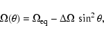
![\begin{displaymath}
{\rm for \ Ca:} \ \ \ \ \Omega (\theta) = 18.870 - 0.872 ~
\sin^2 \theta \ \ \ \ [\hbox{$^\circ$ }/{\rm day}].
\end{displaymath}](/articles/aa/full/2007/09/aa5982-06/img141.gif)
![\begin{displaymath}
{\rm for \ Fe:} \ \ \ \ \Omega (\theta) = 19.183 - 1.019 ~
\sin^2 \theta \ \ \ \ [\hbox{$^\circ$ }/{\rm day}].
\end{displaymath}](/articles/aa/full/2007/09/aa5982-06/img142.gif)
![\begin{figure}
\par\includegraphics[width=8cm,clip]{5982af1.ps}
\end{figure}](/articles/aa/full/2007/09/aa5982-06/img147.gif)