A&A 368, L8-L12 (2001)
DOI: 10.1051/0004-6361:20010145
A. Mazumdar - H. M. Antia
Tata Institute of Fundamental Research,
Homi Bhabha Road, Mumbai 400005, India
Received 2 January 2001 / Accepted 29 January 2001
Abstract
Helioseismic inversions for the rotation rate have established the
presence of a tachocline near the base of the solar convection zone.
We show that the tachocline produces a characteristic
oscillatory signature in the splitting coefficients of low degree
modes, which could be observed on distant stars. Using this
signature it may be possible to determine the characteristics of
the tachocline using only low degree modes. The limitations of
this technique in terms of observational uncertainties are
discussed, to assess the possibility of detecting tachoclines on
distant stars.
Key words: stars: interiors - stars: oscillations - stars: rotation
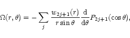
Helioseismic inversions of observed splitting coefficients have enabled us to study the rotation rate inside the Sun (Thompson et al. 1996; Schou et al. 1998). From these inversions it has been established that there is a shear layer near the base of the convection zone where the rotation rate undergoes a transition from differential rotation inside the convection zone to almost uniform rotation in the radiative interior. This layer has been referred to as the tachocline (Spiegel & Zahn 1992). The characteristics of this layer have been studied using helioseismic data (Kosovichev 1996; Basu 1997; Antia et al. 1998; Charbonneau et al. 1999; Corbard et al. 1999). Nevertheless, the origin of this shear layer is not yet clear and it would be instructive to probe the possible existence of these layers in distant stars. Such a study would help us in understanding the formation of tachoclines and to test the theories of angular momentum transport in stellar interiors.
The solar tachocline has been detected using frequency splittings
for modes of low and intermediate degree, ![]() .
All these modes
are not expected to be detected on other stars. In order to
detect a tachocline on distant stars we have to look for the signature
of a tachocline in low degree modes (
.
All these modes
are not expected to be detected on other stars. In order to
detect a tachocline on distant stars we have to look for the signature
of a tachocline in low degree modes (![]() ), which are the
only modes that can be detected on these stars. It has been
shown that rapid variations in the sound speed in the stellar
interior, like those arising at the base of the convection zone
leave a characteristic oscillatory signature in the mean frequencies
of low degree modes (Gough 1990; Monteiro et al. 1994;
Roxburgh & Vorontsov 1994;
Basu et al. 1994).
From this oscillatory signature
it has been possible to put limits on the extent of overshoot
below the solar convection zone (Basu 1997). Monteiro et al.
(2000) have pointed out that this oscillatory signature
can be used to study the location of the base of the convection zone
as well as the extent of overshoot below this base in other stars
using asteroseismic data for only low degree modes.
), which are the
only modes that can be detected on these stars. It has been
shown that rapid variations in the sound speed in the stellar
interior, like those arising at the base of the convection zone
leave a characteristic oscillatory signature in the mean frequencies
of low degree modes (Gough 1990; Monteiro et al. 1994;
Roxburgh & Vorontsov 1994;
Basu et al. 1994).
From this oscillatory signature
it has been possible to put limits on the extent of overshoot
below the solar convection zone (Basu 1997). Monteiro et al.
(2000) have pointed out that this oscillatory signature
can be used to study the location of the base of the convection zone
as well as the extent of overshoot below this base in other stars
using asteroseismic data for only low degree modes.
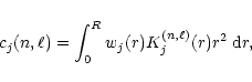
In this work we study the signature of a tachocline in the low degree modes. Since the tachocline is a narrow layer where the rotation rate varies rapidly, we would expect an oscillatory signature in the corresponding splitting coefficients. Using a model for the solar tachocline, we show that this oscillatory signature is indeed present in frequency splitting coefficients of the low degree modes. Further, it is, in principle, possible to determine the characteristics of the tachocline, like its location, width and the extent of variation in the rotation rate across the tachocline using this oscillatory signature.
The frequency
of an eigenmode of a given degree ![]() ,
radial order, n, and
azimuthal order, m can be expressed in
terms of the splitting coefficients, using the expansion
,
radial order, n, and
azimuthal order, m can be expressed in
terms of the splitting coefficients, using the expansion
Following Basu et al. (1994), we take the fourth difference of the splitting coefficients with respect to nto enhance the oscillatory signal. Another advantage of taking the fourth difference is that the smooth part of the splitting coefficients becomes negligible and we do not need to include it in our analysis. This will of course, depend on the smooth component of variation of the rotation rate, but even for a realistic solar rotation profile this component is found to be negligible.
In order to illustrate this oscillatory signature we assume a model
tachocline rotation profile of the form
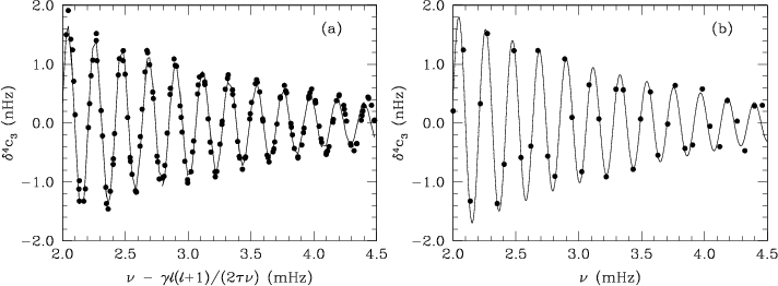 |
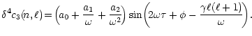
Figure 1:
Fourth difference of the splitting
coefficient c3, for
|
| Open with DEXTER | |
For distant stars it will be possible to detect modes with
![]() only and hence the number of modes will be highly restricted. Even then it is
possible to fit the oscillatory part and Fig. 1b
shows one such fit.
In this case the parameter
only and hence the number of modes will be highly restricted. Even then it is
possible to fit the oscillatory part and Fig. 1b
shows one such fit.
In this case the parameter ![]() is not relevant as the corresponding
term is very small and we fit only the five parameters a0, a1, a2,
is not relevant as the corresponding
term is very small and we fit only the five parameters a0, a1, a2,
![]() and
and ![]() .
All the results presented in this paper are obtained using modes
for
.
All the results presented in this paper are obtained using modes
for
![]() only, unless mentioned otherwise.
only, unless mentioned otherwise.
In order to study the signature of the tachocline in the splitting coefficients
we calculate
![]() with rotation profiles defined by
Eq. (7)
using different values of half-width w, and position
with rotation profiles defined by
Eq. (7)
using different values of half-width w, and position ![]() of the
tachocline. We fit the oscillatory form defined by
Eq. (8) to each of these data sets.
It turns out that the position of the tachocline affects mainly the parameter
of the
tachocline. We fit the oscillatory form defined by
Eq. (8) to each of these data sets.
It turns out that the position of the tachocline affects mainly the parameter
![]() ,
which is close to the acoustic depth of the transition layer.
Therefore, in this work we have only shown results with
,
which is close to the acoustic depth of the transition layer.
Therefore, in this work we have only shown results with
![]() .
Conversely, the location of the tachocline may be determined
from the parameter
.
Conversely, the location of the tachocline may be determined
from the parameter ![]() .
In order to study the effect of width
we use different values of w and the fitted amplitude
(
.
In order to study the effect of width
we use different values of w and the fitted amplitude
(
![]() )
is shown in
Fig. 2. It can be
seen that in all cases the amplitude decreases with increasing
)
is shown in
Fig. 2. It can be
seen that in all cases the amplitude decreases with increasing
![]() ,
which may be expected as the modes with higher frequency
have larger number of nodes in radial direction and hence the
radial wavelength will be smaller, thus giving a smaller contribution
to the integral in Eq. (3).
At larger width the amplitude reduces
and the tachocline profile also gives a contribution to the smooth
part at low frequencies and it is not possible to use the simple
form to fit the data.
It turns out that the extent of
variation in the amplitude across the frequency range depends on the
width of the tachocline. For small width the variation is smaller, while
with increasing width, the variation in amplitude increases. For example,
for
,
which may be expected as the modes with higher frequency
have larger number of nodes in radial direction and hence the
radial wavelength will be smaller, thus giving a smaller contribution
to the integral in Eq. (3).
At larger width the amplitude reduces
and the tachocline profile also gives a contribution to the smooth
part at low frequencies and it is not possible to use the simple
form to fit the data.
It turns out that the extent of
variation in the amplitude across the frequency range depends on the
width of the tachocline. For small width the variation is smaller, while
with increasing width, the variation in amplitude increases. For example,
for
![]() ,
,
![]() ,
,
![]() and
and
![]() ,
the ratios of amplitudes at the two limits in
Fig. 2 are 2.5, 3.0, 5.5 and 100 respectively.
Thus, if we have data covering
the entire frequency range it should be possible to determine the
width using the extent of variation in amplitude. Once the width is
determined, we can determine
,
the ratios of amplitudes at the two limits in
Fig. 2 are 2.5, 3.0, 5.5 and 100 respectively.
Thus, if we have data covering
the entire frequency range it should be possible to determine the
width using the extent of variation in amplitude. Once the width is
determined, we can determine
![]() from the amplitude of the
oscillatory term at the low frequency end. Thus we should be able to
determine the characteristics like position, width and
from the amplitude of the
oscillatory term at the low frequency end. Thus we should be able to
determine the characteristics like position, width and
![]() of the
tachocline using only low degree modes.
of the
tachocline using only low degree modes.
 |
Figure 2:
Comparison of amplitude of oscillatory signal as a function of frequency
for different widths of the transition region for
|
| Open with DEXTER | |
In all the foregoing calculations we have used the exact splitting coefficients
as calculated for a given rotation profile. In real data, there would
naturally be errors associated with each splitting coefficient. In order to
simulate real data we have constructed artificial data sets where
random errors with standard deviation ![]() are added to all the
splitting coefficients. For simplicity, we assume that error is same
in all these coefficients. Using 100 different realizations of errors we
can estimate the expected errors in each of the fitted parameters, the
results of which are summarized in Table 1. For low errors
(
are added to all the
splitting coefficients. For simplicity, we assume that error is same
in all these coefficients. Using 100 different realizations of errors we
can estimate the expected errors in each of the fitted parameters, the
results of which are summarized in Table 1. For low errors
(
![]() nHz) it is
indeed possible to determine all the parameters to reasonable
accuracy and the error in each parameter is proportional to the assumed
error in the splitting coefficients.
nHz) it is
indeed possible to determine all the parameters to reasonable
accuracy and the error in each parameter is proportional to the assumed
error in the splitting coefficients.
| Error ( |
a0 | ||
| (nHz) | (nHz) | (sec) | (rad) |
| 0.010 |
|
|
|
| 0.020 |
|
|
|
| 0.050 |
|
|
|
| 0.100 |
|
|
|
| 0.200 |
|
|
|
| 0.200 |
|
2323 |
|
We have shown that a sharp transition in the rotation rate that is
expected in the tachocline region gives rise to an oscillatory signal in
the splitting coefficients of the low degree modes. The
"wavelength'' of the oscillatory signal is determined by the position
of the tachocline, while the variation in amplitude across the frequency
range is determined by its width. The amplitude of signal is of course
proportional to the extent of the variation in the rotation rate. Thus from
this oscillatory signal it is, in principle,
possible to determine the position,
width and
![]() for the tachocline.
We are looking for the signal in odd splitting coefficients, which can
arise only due to rotation, and not
from magnetic fields or structural variations in the stellar interior.
In this discussion
we have not included any possible latitudinal variation in the
characteristics of the tachocline. The solar tachocline is known
to be prolate (Charbonneau et al. 1999) and this variation would
also affect the oscillatory signal in low degree modes. Using only
low degree modes it may not be possible to disentangle all variations
in the tachocline, but so long as the latitudinal variation is small, as
is the case for the Sun, the mean properties of the tachocline can
be determined from the low degree modes.
for the tachocline.
We are looking for the signal in odd splitting coefficients, which can
arise only due to rotation, and not
from magnetic fields or structural variations in the stellar interior.
In this discussion
we have not included any possible latitudinal variation in the
characteristics of the tachocline. The solar tachocline is known
to be prolate (Charbonneau et al. 1999) and this variation would
also affect the oscillatory signal in low degree modes. Using only
low degree modes it may not be possible to disentangle all variations
in the tachocline, but so long as the latitudinal variation is small, as
is the case for the Sun, the mean properties of the tachocline can
be determined from the low degree modes.
Since the amplitude of the oscillatory signal is very small, it
will be necessary to find the splitting coefficients accurately
to determine the characteristics of the tachocline. From our
simulations it appears that the required accuracy in the splitting
coefficients is ![]() 0.2 nHz for
0.2 nHz for
![]() nHz. Even for the Sun, this level of accuracy
has not been achieved so far and we do not expect it to be achieved for
other stars in near future.
But there is no reason to assume that the variation in rotation
rate in all stars will be comparable to that in the Sun.
In particular, for stars which are fast rotators, we would expect
nHz. Even for the Sun, this level of accuracy
has not been achieved so far and we do not expect it to be achieved for
other stars in near future.
But there is no reason to assume that the variation in rotation
rate in all stars will be comparable to that in the Sun.
In particular, for stars which are fast rotators, we would expect
![]() to be correspondingly larger.
Even for stars with similar rotation rate there may be some
variation in
to be correspondingly larger.
Even for stars with similar rotation rate there may be some
variation in
![]() or in the amplitude of oscillatory signal
for the same
or in the amplitude of oscillatory signal
for the same
![]() .
In this work, all the calculations have been
done for a solar model. In other stars the amplitude may be
somewhat different. If the
star is rotating very rapidly, the linear approximation used to
relate the splitting coefficients to the rotation rate may not
be admissible. But we would expect that for a star which is rotating
about 50 times faster than the Sun, this approximation may still
be applicable and in that case an accuracy of about 10 nHz may be sufficient
to detect the oscillatory signal.
For stars with larger M/R3, this limit may also be larger.
Similarly, if we choose stars with larger differential rotation, or with
favourable amplitude, this number may go up further.
Even if stars are rotating more rapidly the oscillatory signal may
still be present, but mode identification and interpretation may
be more difficult.
The upcoming asteroseismic missions like COROT (Baglin et al. 1998), MOST (Matthews 1998) and MONS
(Kjeldsen & Bedding 1998)
have a planned frequency resolution of 100 nHz, which may not be
sufficient to detect this oscillatory signal.
But with some improvements in instruments and longer observations of
a few selected stars, which are known to be rotating fast
and preferably having larger differential rotation, it may be
possible to detect this signal in not too distant future.
.
In this work, all the calculations have been
done for a solar model. In other stars the amplitude may be
somewhat different. If the
star is rotating very rapidly, the linear approximation used to
relate the splitting coefficients to the rotation rate may not
be admissible. But we would expect that for a star which is rotating
about 50 times faster than the Sun, this approximation may still
be applicable and in that case an accuracy of about 10 nHz may be sufficient
to detect the oscillatory signal.
For stars with larger M/R3, this limit may also be larger.
Similarly, if we choose stars with larger differential rotation, or with
favourable amplitude, this number may go up further.
Even if stars are rotating more rapidly the oscillatory signal may
still be present, but mode identification and interpretation may
be more difficult.
The upcoming asteroseismic missions like COROT (Baglin et al. 1998), MOST (Matthews 1998) and MONS
(Kjeldsen & Bedding 1998)
have a planned frequency resolution of 100 nHz, which may not be
sufficient to detect this oscillatory signal.
But with some improvements in instruments and longer observations of
a few selected stars, which are known to be rotating fast
and preferably having larger differential rotation, it may be
possible to detect this signal in not too distant future.
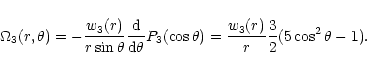
![\begin{displaymath}\Omega(r,\theta)={\delta\Omega (5\cos^2\theta -1)\over
1+\exp[(r_{\rm d}-r)/w]},
\end{displaymath}](/articles/aa/full/2001/11/aada023/img34.gif)