A&A 493, 1029-1041 (2009)
DOI: 10.1051/0004-6361:200810025
V. Agra-Amboage1 - C. Dougados1 - S. Cabrit2 - P. J. V. Garcia3,4,1 - P. Ferruit5
1 - Laboratoire d'Astrophysique de l'Observatoire de
Grenoble, UMR 5521 du CNRS,
38041 Grenoble Cedex, France
2 -
LERMA, Observatoire de Paris, UMR 8112 du
CNRS, 61 avenue de l'Observatoire, 75014 Paris, France
3 -
Departamento de Engenharia Fisica,
Faculdade de Engenharia,
Universidade do Porto
4200-465 Porto, Portugal
4 -
Centro de Astrofisica, Universidade do Porto,
4150-752 Porto, Portugal
5 -
Université de Lyon, 69003 Lyon;
Université de Lyon-1, Observatoire de Lyon, 9 Av. Charles André, 69230
St. Genis Laval; CNRS, UMR 5574, Centre de Recherche d'Astrophysique de Lyon;
École Normale Supérieure de Lyon, 69007 Lyon, France
Received 22 April 2008 / Accepted 21 October 2008
Abstract
Context. High-resolution studies of microjets in T Tauri stars (cTTs) reveal key information on the jet collimation and launching mechanism, but only a handful of systems have been mapped so far.
Aims. We wish to perform a detailed study of the microjet from the 2 ![]() young star RY Tau, to investigate the influence of its higher stellar mass and claimed close binarity on jet properties.
young star RY Tau, to investigate the influence of its higher stellar mass and claimed close binarity on jet properties.
Methods. Spectro-imaging observations of RY Tau were obtained in [O I]![]() 6300 with resolutions of 0
6300 with resolutions of 0
![]() 4 and 135 km s-1, using the integral field spectrograph OASIS at the Canada-France-Hawaii Telescope. Deconvolved images reach a resolution of 0
4 and 135 km s-1, using the integral field spectrograph OASIS at the Canada-France-Hawaii Telescope. Deconvolved images reach a resolution of 0
![]() 2.
2.
Results. The blueshifted jet is detected within 2
![]() of the central star. We determine its PA, collimation, 2D kinematics, mass-flux rate, ejection to accretion ratio, and transverse velocity shifts taking accurately into account errors due to finite signal to noise ratio. The RY Tau system is shown to provide important constraints to several models of steady MHD ejection.
of the central star. We determine its PA, collimation, 2D kinematics, mass-flux rate, ejection to accretion ratio, and transverse velocity shifts taking accurately into account errors due to finite signal to noise ratio. The RY Tau system is shown to provide important constraints to several models of steady MHD ejection.
Conclusions. The remarkably similar properties of the RY Tau microjet compared to jets from lower mass cTTs gives support to the common belief that the jet launching mechanism is universal over a broad range of stellar masses. The proximity between the jet PA and the PA of the photocenter variations observed by Hipparcos calls into question the interpretation of the latter in terms of binarity of RY Tau. Partial occultation events of the photosphere may offer an alternative explanation.
Key words: ISM: jets and outflows - ISM: individual objects: HH 938 - stars: formation - stars: individual: RY Tau - stars: winds, outflows
One of the main open problems in star formation is to understand the physical mechanism by which mass in young stars is ejected from the accreting system and then collimated into jets. Magneto-hydrodynamic accretion-driven wind models best explain the efficient collimation and the large mass ejection efficiencies observed. However, different scenarios are proposed for the origin of the outflow, depending on whether it originates from the stellar surface (Sauty & Tsinganos 1994; Matt & Pudritz 2008), from the inner edge of the accretion disk (Shu et al. 1995), an extended range of disk radii (Casse & Ferreira 2000; Pudritz & Norman 1986), or from reconnexion sites in the stellar magnetosphere (Ferreira et al. 2000; Goodson et al. 1997).
Microjets from T Tauri stars offer a unique opportunity to probe the inner 100 AUs of the outflow where the acceleration and collimation processes occur, and therefore to place strong observational constraints on the ejection mechanism in young stars. Combined kinematic/imaging studies of microjets at sub-arcsecond resolution have allowed major advances in this field in recent years (Ray et al. 2007; Bacciotti et al. 2000; Lavalley et al. 1997; Lavalley-Fouquet et al. 2000, and refs. therein). That the jet phenomenon is very robust over orders of magnitude of central stellar mass is testified by the fact that both brown dwarfs and Herbig Ae/Be stars are known to drive collimated outflows (Corcoran & Ray 1997; Whelan et al. 2005). However, variation of jet properties (collimation, kinematics, mass-loss rates) with mass of the driving source has not yet been investigated in detail. It is thus important to extend the sample of microjets studied at high angular resolution to central sources of differing mass and binary status.
We concentrate here on the intermediate-mass classical T Tauri star
RY Tau, located in the nearby Taurus-Auriga cloud (d = 140 pc).
With spectral type F8-G1 and
![]() (Calvet et al. 2004; Mora et al. 2001), RY Tau is of significantly higher mass than
other nearby atomic jet sources previously spectro-imaged at high
resolution, the most massive so far being RW Aur with 1.4
(Calvet et al. 2004; Mora et al. 2001), RY Tau is of significantly higher mass than
other nearby atomic jet sources previously spectro-imaged at high
resolution, the most massive so far being RW Aur with 1.4 ![]() (Woitas et al. 2001). It thus allows us to probe jet formation in a mass
range intermediate between standard classical T Tauri stars and
Herbig Ae/Be stars (of mass >2
(Woitas et al. 2001). It thus allows us to probe jet formation in a mass
range intermediate between standard classical T Tauri stars and
Herbig Ae/Be stars (of mass >2 ![]() ). The presence of a jet
in RY Tau was indirectly suggested by [O I] emission
blueshifted by -70 km s-1 in its spectrum (Cabrit et al. 1990; Hartigan et al. 1995). It has been recently confirmed by St-Onge & Bastien (2008) who
detected a collimated string of H
). The presence of a jet
in RY Tau was indirectly suggested by [O I] emission
blueshifted by -70 km s-1 in its spectrum (Cabrit et al. 1990; Hartigan et al. 1995). It has been recently confirmed by St-Onge & Bastien (2008) who
detected a collimated string of H![]() emission knots
(HH 938) extending from 1.5
emission knots
(HH 938) extending from 1.5
![]() out to several arcminutes on both
sides of the star. RY Tau is also an active accretor, with veiling
values of
out to several arcminutes on both
sides of the star. RY Tau is also an active accretor, with veiling
values of ![]() 0.1 in the optical (Basri et al. 1991; Hartigan et al. 1995) and 0.8 in the UV (Calvet et al. 2004). The latter corresponds to an updated
accretion rate of
0.1 in the optical (Basri et al. 1991; Hartigan et al. 1995) and 0.8 in the UV (Calvet et al. 2004). The latter corresponds to an updated
accretion rate of
![]()
![]() yr-1, 4 times higher than the previous determination by Hartigan et al. (1995).
yr-1, 4 times higher than the previous determination by Hartigan et al. (1995).
Another important peculiarity of RY Tau besides its mass is a
suspected close binary status from Hipparcos observations. The
variability of the astrometric solution, indicating motion of the
photocentre, is interpreted as indicative of a binary of PA =
![]() and minimum separation of 3.27 AU (Bertout et al. 1999). Such
a close binary companion might have a strong impact on the ability of
the inner disc regions to drive a collimated outflow, possibly leading
to observable differences to microjets from single stars.
and minimum separation of 3.27 AU (Bertout et al. 1999). Such
a close binary companion might have a strong impact on the ability of
the inner disc regions to drive a collimated outflow, possibly leading
to observable differences to microjets from single stars.
In addition to these specific properties, RY Tau shows a remarkably
flat spectral energy distribution in the far-infrared, and a rather
large degree of linear polarisation of a few percent in the optical,
indicating a substantial amount of circumstellar material
(Bastien 1982). RY Tau also shows a peculiar photometric
variability with large variations of brightness accompanied by a near
constancy of colour. Two abrupt brightnening events were recorded in
1983/1984 and 1996/1997 reminiscent of UX Ori events (Petrov et al. 1999; Herbst & Stine 1984). It is also a rapid rotator with a ![]() of
of ![]() km s-1 (Petrov et al. 1999). Petrov et al. (1999) argue that the
photometric behavior can be interpreted as variable obscuration of
the central star by a disc seen at high inclination. The large values
of
km s-1 (Petrov et al. 1999). Petrov et al. (1999) argue that the
photometric behavior can be interpreted as variable obscuration of
the central star by a disc seen at high inclination. The large values
of ![]() and polarisation further support this conclusion.
and polarisation further support this conclusion.
We present in this paper sub-arcsecond optical spectro-imaging observations of the RY Tau microjet in [O I] obtained with the OASIS integral field spectrograph coupled with adaptive optics correction at the Canada France Hawaii telescope. The combination of high angular resolution and intermediate spectral resolution allows for accurate subtraction of the strong central continuum emission, critical to study the inner regions of the jet. Details on the observations and data reduction are given in Sect. 2. In Sect. 3, we discuss the main results regarding the jet morphology, the jet kinematics both along and transverse to the jet axis, the search for rotation signatures and the derivation of mass-loss rates. We analyze these results in the context of previous studies of microjets and discuss their implication for jet launching models and binarity of RY Tau in Sect. 4. We conclude in Sect. 5.
![\begin{figure}
\par\includegraphics[width=8.4cm,clip]{0025fig1.ps}
\end{figure}](/articles/aa/full/2009/03/aa10025-08/img28.gif) |
Figure 1:
Comparison between the EXPORT RY Tau spectrum (thick line,
from Mora et al. 2001) and rotationally broadened EXPORT spectra of
four reference stars (thin lines). The reduced |
| Open with DEXTER | |
Observations of the RY Tau microjet were conducted on January 15th 2002 at the Canada France Hawaii Telescope (CFHT), using the integral
field spectrograph OASIS combined with the adaptive optics system
PUE'O. The configuration used for the RY Tau observations provides a
spectral resolution of
![]() (velocity resolution
(velocity resolution
![]() km s-1 estimated from the width of the [O I] telluric emission
line) and a velocity sampling of 41 km s-1 over a spectral range from
6209 Å to 6549 Å, including the [O
I]6300 Å line. The field of view is 6.2
km s-1 estimated from the width of the [O I] telluric emission
line) and a velocity sampling of 41 km s-1 over a spectral range from
6209 Å to 6549 Å, including the [O
I]6300 Å line. The field of view is 6.2
![]() with a spatial sampling of 0.16
with a spatial sampling of 0.16
![]() per lenslet. After AO correction, the effective spatial resolution
achieved is 0
per lenslet. After AO correction, the effective spatial resolution
achieved is 0
![]() 4 (Gaussian core FWHM). One exposure with
an on-source integration time of 1800 s was obtained.
4 (Gaussian core FWHM). One exposure with
an on-source integration time of 1800 s was obtained.
The data reduction was carried out following the standard OASIS
procedure (Bacon et al. 2001), using the XOasis software. A dedicated
spectral extraction procedure was developed for the OASIS January 2002
run, to correct for a slight rotation of the lenslet array.
Spectro-photometric calibration was performed using the standard star
HD 93521. Final spectra are calibrated in units of 10-19 W m-2 Å
![]() .
Atmospheric
refraction correction was performed a-posteriori by recentering each
spectral image on the continuum centroid, following Garcia et al. (1999).
Subsequent analysis of the data (continuum subtraction, removal of
[O I] sky emission, construction of images and PV diagrams) was
performed under IDL.
.
Atmospheric
refraction correction was performed a-posteriori by recentering each
spectral image on the continuum centroid, following Garcia et al. (1999).
Subsequent analysis of the data (continuum subtraction, removal of
[O I] sky emission, construction of images and PV diagrams) was
performed under IDL.
As Fig. 1 illustrates, the red wing of the [O I] line in RY Tau is strongly distorted by an underlying photospheric absorption line. Therefore, the photospheric spectrum of RY Tau has to be carefully subtracted in order to retrieve the intrinsic jet kinematics and flux close to the source.
Since we did not observe a standard star of similar spectral type as
RY Tau with OASIS, we retrieved from the litterature medium resolution
(R=6600) optical spectra of both RY Tau and standard stars obtained in
the context of the EXPORT project, published in Mora et al. (2001). We
investigated four different reference stars: HD 126053 (G1V), HD 89449
(F6IV), HR 4451 (F8/G0Ib/II) and HR 72 (G0V) to find the best fit to
the continuum. Figure 1 shows the comparison between the
EXPORT spectrum of RY Tau and the photospheric contribution predicted
by the four stars, after rotational broadening by ![]() = 52 km s-1. In accordance with Mora et al. (2001), we find that the best fit is
obtained for HR 4451, of spectral type F8/G0.
= 52 km s-1. In accordance with Mora et al. (2001), we find that the best fit is
obtained for HR 4451, of spectral type F8/G0.
We then developed a dedicated continuum subtraction procedure under
IDL in order to remove the photospheric contribution from our OASIS [O I]![]() 6300 Å spectra at distances
6300 Å spectra at distances
![]() from the star. The EXPORT spectrum of HR 4451 is first rotationally
broadened to the
from the star. The EXPORT spectrum of HR 4451 is first rotationally
broadened to the ![]() of RY Tau and smoothed to the OASIS spectral
resolution. At each lenslet position, this standard spectrum is scaled
to the continuum level in the current OASIS spectrum, as illustrated
in the top-left panel of Fig. 2. It is then subtracted
out, leaving a residual [O I]
of RY Tau and smoothed to the OASIS spectral
resolution. At each lenslet position, this standard spectrum is scaled
to the continuum level in the current OASIS spectrum, as illustrated
in the top-left panel of Fig. 2. It is then subtracted
out, leaving a residual [O I]![]() 6300 Å line
profile essentially free of photospheric features, shown by the solid
curve in the bottom panel of Fig. 2. The good
photospheric subtraction indicates no detectable veiling in our OASIS
spectra, consistent with the low veiling
6300 Å line
profile essentially free of photospheric features, shown by the solid
curve in the bottom panel of Fig. 2. The good
photospheric subtraction indicates no detectable veiling in our OASIS
spectra, consistent with the low veiling ![]() 0.1 in previous
high-resolution optical spectra of RY Tau
(Basri et al. 1991; Hartigan et al. 1995). At larger distances
0.1 in previous
high-resolution optical spectra of RY Tau
(Basri et al. 1991; Hartigan et al. 1995). At larger distances
![]() ,
photospheric absorption lines no longer contribute significantly, and
a simple linear baseline fit to the local continuum over two intervals
on either side of the [O I] line is used, as illustrated in the
top-right panel of Fig. 2. In each residual,
continuum-subtracted spectrum, we also estimate the spectral noise
,
photospheric absorption lines no longer contribute significantly, and
a simple linear baseline fit to the local continuum over two intervals
on either side of the [O I] line is used, as illustrated in the
top-right panel of Fig. 2. In each residual,
continuum-subtracted spectrum, we also estimate the spectral noise
![]() equal to the standard deviation computed over two wavelength
intervals bracketting the [O I] line. This noise estimate thus
takes into account both the original data noise and the uncertainty in
the photospheric continuum subtraction.
equal to the standard deviation computed over two wavelength
intervals bracketting the [O I] line. This noise estimate thus
takes into account both the original data noise and the uncertainty in
the photospheric continuum subtraction.
![\begin{figure}
\par\includegraphics[width=8.4cm,clip]{0025fig2.ps}
\end{figure}](/articles/aa/full/2009/03/aa10025-08/img36.gif) |
Figure 2:
Top panels: solid curves show the observed OASIS [O
I] |
| Open with DEXTER | |
The residual [O I] line emission, especially in the red wing and close to the source, will depend strongly on the estimate of the photospheric line lying underneath. The depth of this absorption feature is seen to vary with the spectral type and/or the luminosity class. However, from the higher resolution spectra obtained by Mora et al. (2001), we see that the depth of the absorption line is well matched by the photospheric spectrum of HR 4451 (Fig. 1). We thus feel confident that our photospheric fitting procedure does not overestimate the red wing of the [O I] line emission close to the source.
[O I] atmospheric line emission is estimated from the average of
13 spectra located at the periphery of the field of view
(
![]() ). It is then subtracted from
each spectrum. This average sky profile is shown with the dotted line
in the bottom panel of Fig. 2. The average peak radial
velocity is -41 km s-1 with respect to RY Tau and the average
peak surface brightness is
). It is then subtracted from
each spectrum. This average sky profile is shown with the dotted line
in the bottom panel of Fig. 2. The average peak radial
velocity is -41 km s-1 with respect to RY Tau and the average
peak surface brightness is
![]() W m-2 Å
W m-2 Å
![]() .
We derive
a velocity resolution of 135 km s-1 from the FWHM of the sky [O
I] line profile. From the lens-to-lens dispersion in the [O
I] sky line centroid velocities (estimated through Gaussian fitting),
we derive a random uncertainty in the velocity calibration of 5 km s-1 (rms). The wavelength scale is converted to a radial velocity
scale with respect to the central source, using a heliocentric radial
velocity for RY Tau of
.
We derive
a velocity resolution of 135 km s-1 from the FWHM of the sky [O
I] line profile. From the lens-to-lens dispersion in the [O
I] sky line centroid velocities (estimated through Gaussian fitting),
we derive a random uncertainty in the velocity calibration of 5 km s-1 (rms). The wavelength scale is converted to a radial velocity
scale with respect to the central source, using a heliocentric radial
velocity for RY Tau of
![]() km s-1(Petrov et al. 1999).
km s-1(Petrov et al. 1999).
![\begin{figure}
\par\includegraphics[width=15cm,clip]{0025fig3.ps}
\end{figure}](/articles/aa/full/2009/03/aa10025-08/img40.gif) |
Figure 3:
Continuum-subtracted [O I] |
| Open with DEXTER | |
Line emission maps in various velocity intervals are reconstructed by
reprojecting the hexagonal OASIS lenslet array onto a square grid with
0
![]() 1 sampling. In the top row of Fig. 3, we display
continuum-subtracted line emission maps in three velocity intervals,
each covering two individual spectral channels of width 41 km s-1: high-velocity blue (HVB): [-137.5: -55.5] km s-1,
low-velocity (LV): [-15.5: +66.5] km s-1, high-velocity red (HVR):
[+66.5: +148.5] km s-1. These intervals are shaded in grey over the
profiles in Fig. 2. The channel centered at -35 km s-1 shows a behavior intermediate between the HVB and LV
intervals. It is thus left out from the channel maps, in order to
better reveal the distinct morphologies between the high and low
velocity ranges.
1 sampling. In the top row of Fig. 3, we display
continuum-subtracted line emission maps in three velocity intervals,
each covering two individual spectral channels of width 41 km s-1: high-velocity blue (HVB): [-137.5: -55.5] km s-1,
low-velocity (LV): [-15.5: +66.5] km s-1, high-velocity red (HVR):
[+66.5: +148.5] km s-1. These intervals are shaded in grey over the
profiles in Fig. 2. The channel centered at -35 km s-1 shows a behavior intermediate between the HVB and LV
intervals. It is thus left out from the channel maps, in order to
better reveal the distinct morphologies between the high and low
velocity ranges.
The continuum map, computed by integration of the estimated
photospheric contribution over the velocity interval [-2400, -500 km s-1], is also shown in the last top panel. Fitting the brightness
radial distribution of the continuum map with a Moffat function,
representative of a partially corrected AO point-spread function
(PSF), gives a Gaussian core width of
![]() .
We determine
the centroid continuum position with an accuracy (1
.
We determine
the centroid continuum position with an accuracy (1![]() )
of
0
)
of
0
![]() 015 from 2D Gaussian fitting. In all figures, spatial offsets are
plotted relative to this continuum centroid.
015 from 2D Gaussian fitting. In all figures, spatial offsets are
plotted relative to this continuum centroid.
In the HVB map, tracing high blueshifted velocities, the [O I] jet emission is clearly detected out to distances of 2
![]() towards the north-west. The line emission peak is slightly displaced
along the jet from the continuum centroid position (
towards the north-west. The line emission peak is slightly displaced
along the jet from the continuum centroid position (
![]() ,
,
![]() )
and the emission is
resolved (
)
and the emission is
resolved (
![]() ). In the LV map, tracing low flow
velocities, the emission is marginally resolved (
). In the LV map, tracing low flow
velocities, the emission is marginally resolved (
![]() )
and
centered closer to the continuum position (
)
and
centered closer to the continuum position (
![]() 032,
032,
![]() 018). At high redshifted
velocities (HVR map), the emission is dominated by an unresolved
component (
018). At high redshifted
velocities (HVR map), the emission is dominated by an unresolved
component (
![]() 4) centered on the continuum position
within positional uncertainties (
4) centered on the continuum position
within positional uncertainties (
![]() 025,
025,
![]() 016). Some low level
extended emission also appears towards the east. This extension is
also faintly present in the LV map, although its relative contribution
is much less important. We checked that this residual redshifted
emission remains when using another reference star for the
photospheric emission subtraction. This extended component shows a
position angle significantly different from the one of the blueshifted
jet emission and might trace strong brightness asymmetry in the
counter-jet emission. However this feature has a low signal to noise
ratio (between 3 and 5, see Fig. 3), thus preventing us from
a detailed analysis of its possible origin.
016). Some low level
extended emission also appears towards the east. This extension is
also faintly present in the LV map, although its relative contribution
is much less important. We checked that this residual redshifted
emission remains when using another reference star for the
photospheric emission subtraction. This extended component shows a
position angle significantly different from the one of the blueshifted
jet emission and might trace strong brightness asymmetry in the
counter-jet emission. However this feature has a low signal to noise
ratio (between 3 and 5, see Fig. 3), thus preventing us from
a detailed analysis of its possible origin.
In order to remove the non Gaussian wings of the partially
corrected AO PSF and derive accurate estimates of jet position angle
and jet emission widths, we have deconvolved the observed channel
maps, using the continuum map as an estimate of the corresponding
point spread function. We use the LUCY restoration routine as
implemented in the STSDAS/IRAF package. We limit ourselves to 20-25 iterations (standard acceleration method) which yield ![]() values
of 1.4, 1.1, 2.0 for the 3 channels respectively and final resolution
of
values
of 1.4, 1.1, 2.0 for the 3 channels respectively and final resolution
of
![]() 2 (estimated by fitting a Gaussian profile to
the central compact component in the HVR map). The maximum number
of iterations was determined by ensuring that the derived image
characteristics (such as intrinsic jet FWHM) did not change
significantly with further iterations. The deconvolved maps are shown
in the bottom panels of Fig. 3.
2 (estimated by fitting a Gaussian profile to
the central compact component in the HVR map). The maximum number
of iterations was determined by ensuring that the derived image
characteristics (such as intrinsic jet FWHM) did not change
significantly with further iterations. The deconvolved maps are shown
in the bottom panels of Fig. 3.
As already noticed in the raw maps, the line emission is dominated in
all channels by a compact component very close to the star. It is
unresolved and centered at the continuum position in the HVR map, and
shows increasing FWHM and spatial offset towards more blueshifted
velocities. The extended jet emission stands out more clearly in the
deconvolved HVB map, with the low-level emission in the raw map
sharpening into an emission knot located at
![]() 23,
23,
![]() 55, ie at a distance of
55, ie at a distance of
![]() (190 AU) from the star. In the HVR map, the low
level extension towards the east stands out clearly (at a level of 0.2% of the peak emission).
(190 AU) from the star. In the HVR map, the low
level extension towards the east stands out clearly (at a level of 0.2% of the peak emission).
From the HVB deconvolved map, we derive a position angle (PA) for the
blueshifted jet of 294
![]() .
This orientation agrees
with the mean of the PA values of 292
.
This orientation agrees
with the mean of the PA values of 292
![]() derived on
larger scales for H
derived on
larger scales for H![]() knots by St-Onge & Bastien (2008). Our
derived blueshifted jet PA is perpendicular to the direction of the
velocity gradient in interferometric millimetric CO maps or RY Tau,
knots by St-Onge & Bastien (2008). Our
derived blueshifted jet PA is perpendicular to the direction of the
velocity gradient in interferometric millimetric CO maps or RY Tau,
![]()
![]() (Koerner & Sargent 1995), indicating that the jet is
parallel to the spin axis of the disk. It is also perpendicular to
the average direction of the optical linear polarization vector
derived by Bastien (1982) of 20
(Koerner & Sargent 1995), indicating that the jet is
parallel to the spin axis of the disk. It is also perpendicular to
the average direction of the optical linear polarization vector
derived by Bastien (1982) of 20
![]() .
Interestingly, the
derived jet PA is also compatible with the direction of the
photocenter variation seen by Hipparcos (
.
Interestingly, the
derived jet PA is also compatible with the direction of the
photocenter variation seen by Hipparcos (
![]() ), interpreted as the direction to a possible binary
companion (Bertout et al. 1999). We will return to this issue in the
discussion section.
), interpreted as the direction to a possible binary
companion (Bertout et al. 1999). We will return to this issue in the
discussion section.
![\begin{figure}
\par\includegraphics[angle=270,width=8.4cm,clip]{0025fig4.ps}
\end{figure}](/articles/aa/full/2009/03/aa10025-08/img59.gif) |
Figure 4:
Large filled circles: PSF-corrected width
( FWHM) of the RY Tau jet forbidden line emission versus projected
distance from the star, as derived from the [O I] HVB deconvolved map (see text). Measurements available on the same
spatial scales for other TTS microjets are also plotted with various
symbols, after correction for the corresponding PSF. The
object-symbol correspondance and references are given at the top
left corner of the plot. The position of the knot located at
|
| Open with DEXTER | |
We show in Fig. 4 the variation of the intrinsic jet
width as a function of the distance to the star. We estimate the
intrinsic jet width as:
![]() ,
where
FWHM is measured from Gaussian fits to the 1D transverse jet emission
profiles in the deconvolved HVB map, of effective resolution
,
where
FWHM is measured from Gaussian fits to the 1D transverse jet emission
profiles in the deconvolved HVB map, of effective resolution
![]() .
The RY Tau jet width increases slowly from 0
.
The RY Tau jet width increases slowly from 0
![]() 2
(28 AU) at projected distances 0
2
(28 AU) at projected distances 0
![]() 6
(20-84 AU) to 0
6
(20-84 AU) to 0
![]() 3 (42 AU) at
3 (42 AU) at
![]() (280 AU) with a
full opening angle of
(280 AU) with a
full opening angle of ![]() 5
5
![]() .
This behavior is remarkably
similar to that of other T Tauri microjets observed at sub-arcsecond
resolution (see Fig. 4 and discussion
section). We do not see any clear change of jet
width at the location of the knot (projected distance along the jet of 190 AU), within our angular resolution.
.
This behavior is remarkably
similar to that of other T Tauri microjets observed at sub-arcsecond
resolution (see Fig. 4 and discussion
section). We do not see any clear change of jet
width at the location of the knot (projected distance along the jet of 190 AU), within our angular resolution.
![\begin{figure}
\par\includegraphics[width=8.4cm,clip]{0025fg5a.ps}\par\vspace*{2mm}
\includegraphics[width=8.4cm,clip]{0025fg5b.ps}
\end{figure}](/articles/aa/full/2009/03/aa10025-08/img65.gif) |
Figure 5:
Maps of the centroid radial velocity ( top) and
velocity width ( bottom) of a one-component Gaussian fit to the
[OI] |
| Open with DEXTER | |
High spectral resolution integrated line profiles of [O I] in RY Tau show two distinct kinematical components, a high-velocity component (HVC) with peak radial velocities of -70, -80 km s-1 and a low-velocity component (LVC) peaked at -4 km s-1(Hirth et al. 1997; Hartigan et al. 1995). Since both components contribute close to the star, we first tried to perform two-component Gaussian fits to each individual OASIS line profile. However, because of insufficient spectral resolution, the two velocity components cannot be well separated in our data (see bottom panel of Fig. 2) and a globally consistent fit could not be found over the whole field of view.
To obtain an overall view of the 2D kinematics of the RY Tau jet, we
thus performed a single-component Gaussian fit to our spectra. We
show in Fig. 5 the resulting maps of centroid velocity and
profile FWHM. We overlay on these maps the contours of the signal to noise
ratio (SNR) at the line peak. Note that due to combined strong photon
noise and strong residuals of photospheric subtraction close to
the central source, the maximum peak SNR is not reached at the star
position but towards the blueshifted jet. In photon noise statistics,
and for an infinite sampling, the standard deviation of the centroid
estimate for a Gaussian distribution of rms standard deviation
![]() and peak signal-to-noise SNR is given by:
and peak signal-to-noise SNR is given by:
![]() (Porter et al. 2004).
Uncertainties in line centroid velocities derived from our Gaussian
fitting procedure are thus typically:
(Porter et al. 2004).
Uncertainties in line centroid velocities derived from our Gaussian
fitting procedure are thus typically:
![]() ,
i.e.
,
i.e. ![]() 11-16 km s-1 for a line peak
11-16 km s-1 for a line peak
![]() and a line FWHM ranging from 135 to 200 km s-1typical of our observations.
and a line FWHM ranging from 135 to 200 km s-1typical of our observations.
The centroid map shows that the extended blueshifted jet emission at
![]() has centroid velocities of average value
-70 km s-1, consistent with the HVC in previous high-spectral
resolution observations. The jet shows a local peak in centroid
velocity (-90 km s-1) at
has centroid velocities of average value
-70 km s-1, consistent with the HVC in previous high-spectral
resolution observations. The jet shows a local peak in centroid
velocity (-90 km s-1) at
![]() (
(
![]() 2, +0
2, +0
![]() 6), coincident with the emission knot
identified in the deconvolved HVB channel map (denoted with an
asterisk in Fig. 5). The profile width is narrow, and
essentially unresolved beyond
6), coincident with the emission knot
identified in the deconvolved HVB channel map (denoted with an
asterisk in Fig. 5). The profile width is narrow, and
essentially unresolved beyond
![]() from the star.
from the star.
Closer to the star, centroid velocities progressively decrease to values of ![]() -30, -10 km s-1 while the line FWHM significantly increases. The
available velocity information combined with the channel maps from
Fig. 3 suggests that, towards the central source, emission
from the spatially unresolved LVC component at -4 km s-1centered at the continuum position strongly contributes to the line profile,
resulting in intermediate centroid velocities and increased line widths.
-30, -10 km s-1 while the line FWHM significantly increases. The
available velocity information combined with the channel maps from
Fig. 3 suggests that, towards the central source, emission
from the spatially unresolved LVC component at -4 km s-1centered at the continuum position strongly contributes to the line profile,
resulting in intermediate centroid velocities and increased line widths.
In a small zone on the redshifted side, at
![]() (+0
(+0
![]() 8, -0
8, -0
![]() 3), peak velocities appear
slightly redshifted and line profiles become significantly broader
with a fitted
3), peak velocities appear
slightly redshifted and line profiles become significantly broader
with a fitted
![]() km s-1, corresponding to an
intrinsic
km s-1, corresponding to an
intrinsic
![]() km s-1, suggesting a contribution from a
third kinematical component. This region spatially coincides with the
red extension identified in the reconstructed HVR channel map from
Fig. 3.
km s-1, suggesting a contribution from a
third kinematical component. This region spatially coincides with the
red extension identified in the reconstructed HVR channel map from
Fig. 3.
![\begin{figure}
\par\includegraphics[width=7.4cm,clip]{0025fig6.ps}
\end{figure}](/articles/aa/full/2009/03/aa10025-08/img78.gif) |
Figure 6:
Position-velocity map along the RY Tau jet in [O
I] |
| Open with DEXTER | |
Figure 6 shows a position-velocity map along the jet in [O I], reconstructed by averaging the lenslets transversally
across a 1
![]() wide pseudo-slit, and sampling every 0
wide pseudo-slit, and sampling every 0
![]() 2
along the jet. Centroid velocities derived from one-component
Gaussian fits to the line profiles are also plotted. Beyond 0
2
along the jet. Centroid velocities derived from one-component
Gaussian fits to the line profiles are also plotted. Beyond 0
![]() 5, we clearly detect the high-velocity blue jet (HVC) with
an average centroid radial velocity of
5, we clearly detect the high-velocity blue jet (HVC) with
an average centroid radial velocity of ![]() -70 km s-1. The
profiles are essentially unresolved spectrally in the jet (
-70 km s-1. The
profiles are essentially unresolved spectrally in the jet (
![]() km s-1). Average variations in radial velocities along the
blue jet do not exceed 10% (7 km s-1) beyond 0
km s-1). Average variations in radial velocities along the
blue jet do not exceed 10% (7 km s-1) beyond 0
![]() 6 over
the central 2
6 over
the central 2
![]() 5. Closer to the star, centroid radial
velocities progressively decrease and converge to
5. Closer to the star, centroid radial
velocities progressively decrease and converge to ![]()
![]() on the redshifted side, consistent with the
LVC. The lines become asymmetric and wider with an intrinsic FWHM
(deconvolved from the instrumental
on the redshifted side, consistent with the
LVC. The lines become asymmetric and wider with an intrinsic FWHM
(deconvolved from the instrumental
![]() km s-1) of
km s-1) of ![]() 130 km s-1 (see profile in bottom panel of
Fig. 2).
130 km s-1 (see profile in bottom panel of
Fig. 2).
![\begin{figure}
\par\includegraphics[width=8.2cm,clip]{0025fig7.ps}
\end{figure}](/articles/aa/full/2009/03/aa10025-08/img81.gif) |
Figure 7:
Transverse position-velocity diagrams across the blue jet
at distances of 0
|
| Open with DEXTER | |
We show in Fig. 7 transverse position-velocity maps
reconstructed by integrating spectra within a 0
![]() 2 wide pseudo
slit positioned perpendicular to the jet axis at two different
distances from the star along the jet axis. These two
position-velocity diagrams illustrate the transverse structure of the
jet. Close to the source (at
2 wide pseudo
slit positioned perpendicular to the jet axis at two different
distances from the star along the jet axis. These two
position-velocity diagrams illustrate the transverse structure of the
jet. Close to the source (at
![]() 4), where the LVC component
still marginally contributes, the emission on the jet axis peaks at
intermediate velocities (-60 km s-1) and is marginally resolved
transversally. At
4), where the LVC component
still marginally contributes, the emission on the jet axis peaks at
intermediate velocities (-60 km s-1) and is marginally resolved
transversally. At
![]() 2, the emission is more resolved
transversally and the radial velocities peak at -80 km s-1towards the jet axis, consistent with the HVC component. In both
cases, radial velocities decrease by 20 km s-1 in the external
parts of the jet at transverse distances +/-0
2, the emission is more resolved
transversally and the radial velocities peak at -80 km s-1towards the jet axis, consistent with the HVC component. In both
cases, radial velocities decrease by 20 km s-1 in the external
parts of the jet at transverse distances +/-0
![]() 6.
6.
Transverse velocity gradients, indicative of possible rotation within the jet body, have been previously reported for 5 TTS microjets (Bacciotti et al. 2002; Coffey et al. 2007; Woitas et al. 2005; Coffey et al. 2004).
The principle of the measurement of rotation is to search for
radial velocity differences between pairs of spectra emitted at two
symmetrical transverse offsets ![]()
![]() on either side of the
jet axis. In an axisymmetric flow, these velocity differences
on either side of the
jet axis. In an axisymmetric flow, these velocity differences
![]() would be related to the rotation
velocity by
would be related to the rotation
velocity by
![]() ,
where i is
the inclination of the jet axis to the line of sight, provided
,
where i is
the inclination of the jet axis to the line of sight, provided
![]() is larger than the telescope
PSF and on the order of the jet emission radius, to
minimize convolution and projection effects (Pesenti et al. 2004).
is larger than the telescope
PSF and on the order of the jet emission radius, to
minimize convolution and projection effects (Pesenti et al. 2004).
The RY Tau transverse position-velocity diagrams presented in
Fig. 7 do show a skewness in the outer contours
indicative of transverse velocity gradients.
Velocity shifts between
two spectra can be measured either by the difference of the
centroid velocities (determined by fitting a Gaussian profile to
each line) or directly by cross-correlating the two profiles. We
apply both methods to compute transverse velocity shifts
at various transverse distances to the jet axis
(![]() )
and distances from the central source along the jet axis
(d//). We first averaged lenslets over boxes
of width 0
)
and distances from the central source along the jet axis
(d//). We first averaged lenslets over boxes
of width 0
![]() 4 along the jet and
0
4 along the jet and
0
![]() 2 across the jet, in order to increase the signal to noise ratio
and to decrease the random wavelength calibration uncertainty (typically with 3-4 lenslets per box, the latter is down to
2 across the jet, in order to increase the signal to noise ratio
and to decrease the random wavelength calibration uncertainty (typically with 3-4 lenslets per box, the latter is down to
![]() km s-1).
The results are shown in Fig. 8 for
km s-1).
The results are shown in Fig. 8 for
![]() and
and
![]() .
Computed velocity
shifts range between -10 km s-1 and +10 km s-1 for
.
Computed velocity
shifts range between -10 km s-1 and +10 km s-1 for
![]() ,
and between -35 km s-1 and +15 km s-1 for
,
and between -35 km s-1 and +15 km s-1 for
![]() ,
and show
no clear trend with distance along the jet axis.
,
and show
no clear trend with distance along the jet axis.
The random errors due to noise associated with our transverse velocity
shift measurements are assessed through a Monte-Carlo study detailed
in Appendix A. We show that the Gaussian fitting method is more
accurate, and that the uncertainties associated with our velocity
shifts measurements are well represented by the empirical formula
![]() km s-1, as expected
theoretically for our typical line width (Porter et al. 2004). Based on
the above formula, we thus expect a 1
km s-1, as expected
theoretically for our typical line width (Porter et al. 2004). Based on
the above formula, we thus expect a 1![]() uncertainty in velocity
shifts derived from Gaussian fits of
uncertainty in velocity
shifts derived from Gaussian fits of ![]() 4 km s-1 for peak
4 km s-1 for peak
![]() ,
and
,
and ![]() 8.5 km s-1 for peak
8.5 km s-1 for peak
![]() (significantly larger than wavelength calibration errors). Of course
these estimates are only valid as long as the observed profiles do not
depart too much from a Gaussian profile, which is our case in the
blueshifted jet of RY Tau. Otherwise, the cross-correlation technique
should be preferred for measuring velocity shifts and the
corresponding uncertainties will be larger (see Appendix A). For
completeness, both the Gaussian centroid and the correlation method
are shown here, and they give identical results.
(significantly larger than wavelength calibration errors). Of course
these estimates are only valid as long as the observed profiles do not
depart too much from a Gaussian profile, which is our case in the
blueshifted jet of RY Tau. Otherwise, the cross-correlation technique
should be preferred for measuring velocity shifts and the
corresponding uncertainties will be larger (see Appendix A). For
completeness, both the Gaussian centroid and the correlation method
are shown here, and they give identical results.
The 3![]() error-bars derived from the profile SNR using the above
empirical formula from our Monte-Carlo study are plotted in
Fig. 8, for each transverse velocity difference. The
detected velocity shifts at
error-bars derived from the profile SNR using the above
empirical formula from our Monte-Carlo study are plotted in
Fig. 8, for each transverse velocity difference. The
detected velocity shifts at
![]()
![]() are all
compatible with zero (at the 3
are all
compatible with zero (at the 3![]() level), as expected from
beam-convolution effects. Indeed, for transverse distances
significantly smaller than the spatial PSF, contributions to rotation
signatures from receding and approaching flow lines should cancel out
in the beam (Pesenti et al. 2004).
level), as expected from
beam-convolution effects. Indeed, for transverse distances
significantly smaller than the spatial PSF, contributions to rotation
signatures from receding and approaching flow lines should cancel out
in the beam (Pesenti et al. 2004).
For transverse distances of the order of the jet width and larger than
our spatial resolution (
![]() 6) where rotation
signatures should be optimized (Pesenti et al. 2004), the detected
velocity shifts are also compatible everywhere with zero except
marginally at two distances along the jet axis:
6) where rotation
signatures should be optimized (Pesenti et al. 2004), the detected
velocity shifts are also compatible everywhere with zero except
marginally at two distances along the jet axis:
![]() 4
and
4
and
![]() 2 where we detect at a 2.5-3
2 where we detect at a 2.5-3![]() level
transverse velocity shifts of
level
transverse velocity shifts of
![]() of
of
![]() km s-1 and -
km s-1 and -
![]() km s-1 respectively. These transverse asymmetries in
velocities are clearly visible on the two transverse position-velocity
diagrams shown in Fig. 7, which correspond to
these same two distances from the source. We discuss in
Sect. 4.3 whether or not these two marginally detected
velocity shifts could trace signatures of rotation within the jet
body.
km s-1 respectively. These transverse asymmetries in
velocities are clearly visible on the two transverse position-velocity
diagrams shown in Fig. 7, which correspond to
these same two distances from the source. We discuss in
Sect. 4.3 whether or not these two marginally detected
velocity shifts could trace signatures of rotation within the jet
body.
![\begin{figure}
\par\includegraphics[width=8.4cm,clip]{0025fig8.ps}
\end{figure}](/articles/aa/full/2009/03/aa10025-08/img98.gif) |
Figure 8:
Top and middle panels: velocity shifts between
symmetric spectra taken at |
| Open with DEXTER | |
We estimate the mass-loss rate in the blueshifted jet from the [O
I] line luminosities using two different methods described in
detail by Hartigan et al. (1995), hereafter HEG95, and
Cabrit (2002). The first method assumes volume emission over the
entire elementary aperture under uniform plasma conditions (![]() ,
,
![]() ,
,![]() =
= ![]() /
/![]() ). The mass-loss rate is then expressed as:
). The mass-loss rate is then expressed as:
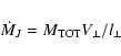 |
(1) |
![\begin{displaymath}M_{\rm TOT}=9.61 \times
10^{-6} \left(\frac{1}{1-x_{\rm e}}\...
...ht)
\left(\frac{L_{\rm [OI]~6300}}{L_{\odot}}\right)M_{\odot}
\end{displaymath}](/articles/aa/full/2009/03/aa10025-08/img107.gif) |
(2) |
The second method assumes that [O I] line emission within each
elementary aperture arises from shock fronts. The mass-loss
rate is then expressed as a function of the shock velocity as:
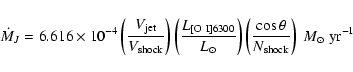 |
(3) |
By comparing the above two methods applied to stellar jets observed
with both small and large apertures, Cabrit (2002) concluded that
on average
![]() /
/
![]()
![]() per 100 AU of jet
length. We will thus assume a value of 1 here for this ratio (our flux
apertures have
per 100 AU of jet
length. We will thus assume a value of 1 here for this ratio (our flux
apertures have
![]() AU along the jet, see below). We
will adopt a jet speed of
AU along the jet, see below). We
will adopt a jet speed of
![]() = 165 km s-1, and a
tangential velocity
= 165 km s-1, and a
tangential velocity
![]() km s-1, corresponding to a
blue jet inclination to the line of sight of 65
km s-1, corresponding to a
blue jet inclination to the line of sight of 65![]() (see Sect. 4.1 for estimates of the RY Tau jet inclination).
(see Sect. 4.1 for estimates of the RY Tau jet inclination).
Since our present dataset of RY Tau only includes the [O I] line, values of ![]() ,
,
![]() ,
and
,
and
![]() cannot be inferred
directly from [S II] and [N II] line ratios, as done
previously in our OASIS study of the DG Tau microjet
(Lavalley-Fouquet et al. 2000) and we have to rely on estimates. We note
that low shock velocities are expected from the non-detection of [N II] emission in RY Tau (Hirth et al. 1997; Hartigan et al. 1995). Indeed,
planar shock models predict a sharp decrease of emissivity for this
line for shock velocities below 30 km s-1 (Hartigan et al. 1994). We
may thus assume in Eq. (3) that
cannot be inferred
directly from [S II] and [N II] line ratios, as done
previously in our OASIS study of the DG Tau microjet
(Lavalley-Fouquet et al. 2000) and we have to rely on estimates. We note
that low shock velocities are expected from the non-detection of [N II] emission in RY Tau (Hirth et al. 1997; Hartigan et al. 1995). Indeed,
planar shock models predict a sharp decrease of emissivity for this
line for shock velocities below 30 km s-1 (Hartigan et al. 1994). We
may thus assume in Eq. (3) that
![]() is in the range 20 to 50 km s-1. For
is in the range 20 to 50 km s-1. For ![]() and
and ![]() in Eq. (2), we will adopt typical
parameters inferred from high-angular resolution observations of the inner
regions of the DG Tau, RW Aur, Th 28 and HH 30 microjets
(Hartigan & Morse 2007; Dougados et al. 2002; Lavalley-Fouquet et al. 2000; Bacciotti & Eislöffel 1999). We thus assume
an ionisation fraction
in Eq. (2), we will adopt typical
parameters inferred from high-angular resolution observations of the inner
regions of the DG Tau, RW Aur, Th 28 and HH 30 microjets
(Hartigan & Morse 2007; Dougados et al. 2002; Lavalley-Fouquet et al. 2000; Bacciotti & Eislöffel 1999). We thus assume
an ionisation fraction ![]() = 10 % and an electronic density
decreasing with distance to the central source as
= 10 % and an electronic density
decreasing with distance to the central source as ![]()
![]() cm-3 for
cm-3 for ![]() AU, and flattening to a
constant value of
AU, and flattening to a
constant value of
![]() cm-3 inside 60 AU
(Hartigan & Morse 2007).
cm-3 inside 60 AU
(Hartigan & Morse 2007).
We estimate the blueshifted HVC jet [O I] luminosities at
different distances along the jet axis by integrating observed surface
brightnesses over the 3 velocity channels centered at -117, -76 and -35 km s-1 (i.e. a total velocity range from -137.5 to -14.5 km s-1 taking into account the channel width). We now include the
spectral channel centered at -35 km s-1 since it always contains
a significant fraction of the total HVC flux, due to our moderate
spectral resolution (see Fig. 2). The emission is summed
in the raw maps over rectangular apertures of full longitudinal
and transverse widths of 0
![]() and 1
and 1
![]() respectively. The chosen longitudinal width provides a
sampling along the jet axis similar to our spatial PSF, while the
full transverse width ensures that we include all of the jet emission
over our field of view (measured transverse
respectively. The chosen longitudinal width provides a
sampling along the jet axis similar to our spatial PSF, while the
full transverse width ensures that we include all of the jet emission
over our field of view (measured transverse
![]() in
our raw maps for distances along the jet axis
in
our raw maps for distances along the jet axis ![]() 2
2
![]() ). The
derived HVC [O I] luminosities as a function of projected
distance along the jet axis are plotted in Fig. 9. We
observe a steep decrease in brightness with distance from the source,
reaching two orders of magnitude at 2.5
). The
derived HVC [O I] luminosities as a function of projected
distance along the jet axis are plotted in Fig. 9. We
observe a steep decrease in brightness with distance from the source,
reaching two orders of magnitude at 2.5
![]() .
However, within
0
.
However, within
0
![]() 6 from the central source, the measured [O I] luminosities are strongly contaminated by the strong low-velocity
component, as indicated by centroid velocities lower than -70 km s-1 (see Fig. 6). Beyond distances of 2
6 from the central source, the measured [O I] luminosities are strongly contaminated by the strong low-velocity
component, as indicated by centroid velocities lower than -70 km s-1 (see Fig. 6). Beyond distances of 2
![]() ,
part of the transverse aperture falls outside the OASIS observations
field of view. Distances between 0
,
part of the transverse aperture falls outside the OASIS observations
field of view. Distances between 0
![]() 6 and 1
6 and 1
![]() 8 from the star
(hereafter denoted as the HVC-dominated region) thus give the best
estimate of the HVC jet luminosity.
8 from the star
(hereafter denoted as the HVC-dominated region) thus give the best
estimate of the HVC jet luminosity.
We also plot in Fig. 9 our estimates of mass-loss
rates using the methods of volume (Eq. (2)) and shock (Eq. (3))
emission. Since we assume for simplicity a constant value of shock
speed and
![]() /
/
![]() = 1, and since
= 1, and since
![]() also remains
constant within 10% along the jet, the mass-flux rate we derive from
the shock method is exactly proportional to the [O I] luminosity
(see Eq. (3)) and thus follows the same steep decrease with distance to
the central star. In particular, it drops by a factor of 5 from the d
= 0.8'' to the d=1.6'' apertures covering the HVC-dominated region.
Although a real variation in
also remains
constant within 10% along the jet, the mass-flux rate we derive from
the shock method is exactly proportional to the [O I] luminosity
(see Eq. (3)) and thus follows the same steep decrease with distance to
the central star. In particular, it drops by a factor of 5 from the d
= 0.8'' to the d=1.6'' apertures covering the HVC-dominated region.
Although a real variation in
![]() of this magnitude cannot be
completely ruled out a priori over a time span of 4 yrs (crossing time
of the HVC-dominated region), we suspect that this drop is mainly an
artefact of our simplifying assumptions in the shock method. Our
argument is that all TTS microjets images at sub-arcsecond
resolution so far show a strongly decreasing [O I] jet
luminosity over their inner 200 AU; If this decrease were proportional
to a jet mass-flux variation, one would expect to also encounter stars
with rising jet brightness over the same distance scales, whereas none
have been seen. Therefore, the jet mass-flux is probably not strictly
proportional to the jet luminosity over the jet length, and the factor
5 decline obtained by the shock method for a constant
of this magnitude cannot be
completely ruled out a priori over a time span of 4 yrs (crossing time
of the HVC-dominated region), we suspect that this drop is mainly an
artefact of our simplifying assumptions in the shock method. Our
argument is that all TTS microjets images at sub-arcsecond
resolution so far show a strongly decreasing [O I] jet
luminosity over their inner 200 AU; If this decrease were proportional
to a jet mass-flux variation, one would expect to also encounter stars
with rising jet brightness over the same distance scales, whereas none
have been seen. Therefore, the jet mass-flux is probably not strictly
proportional to the jet luminosity over the jet length, and the factor
5 decline obtained by the shock method for a constant
![]() and
and
![]() is an upper limit to the true variation in
is an upper limit to the true variation in
![]() (e.g.,
(e.g.,
![]() and
and
![]() could easily decrease with distance from
the star in a time-variable jet, causing a luminosity decline even for
a constant mass-flux; see Eq. (3)).
could easily decrease with distance from
the star in a time-variable jet, causing a luminosity decline even for
a constant mass-flux; see Eq. (3)).
![\begin{figure}
\par\includegraphics[width=8.4cm,clip]{0025fig9.ps} \end{figure}](/articles/aa/full/2009/03/aa10025-08/img129.gif) |
Figure 9:
Mass-loss rate in the RY Tau blueshifted jet as a function
of projected distance, derived from the [O I] line luminosity
with two different assumptions (see text): volume emission (
dot-dashed line) and shock layer with shock speed 20 km s-1 ( red long-dashed line) or 50 km s-1 ( blue short-dashed
line). The two methods are in good agreement in the region
dominated by the HV component. The [O I] line luminosity,
integrated over apertures of
|
| Open with DEXTER | |
In support of this conclusion, we note that the volume method gives
values that are much more uniform along the jet, because the decline
in [O I] luminosity is now compensated for by the drop of ![]() (see Eq. (2)). Across the HVC-dominated region, values of the mass-loss
rate derived by this method change by only a factor 2, and are well
bracketed by the shock method for low to intermediate shock speeds
(20-50 km s-1). We thus take the average volume method mass-loss
rate over distances of 0
(see Eq. (2)). Across the HVC-dominated region, values of the mass-loss
rate derived by this method change by only a factor 2, and are well
bracketed by the shock method for low to intermediate shock speeds
(20-50 km s-1). We thus take the average volume method mass-loss
rate over distances of 0
![]() 6-1
6-1
![]() 8 from the star of
8 from the star of
![]()
![]() yr-1 as our best estimate of the mean HVC
mass-loss rate. The uncertainty on the jet velocity (see below), and
on the typical electronic densities at projected distances 100-150 AU,
suggests an uncertainty of at most a factor of 4 either way,
consistent with the good agreement with the shock methods noted
above. The mass-loss rate in the RY Tau blueshifted jet therefore
is between 0.16 and
yr-1 as our best estimate of the mean HVC
mass-loss rate. The uncertainty on the jet velocity (see below), and
on the typical electronic densities at projected distances 100-150 AU,
suggests an uncertainty of at most a factor of 4 either way,
consistent with the good agreement with the shock methods noted
above. The mass-loss rate in the RY Tau blueshifted jet therefore
is between 0.16 and
![]()
![]() yr-1. Combining with the range of disc mass accretion
rates determined by Calvet et al. (2004) of
yr-1. Combining with the range of disc mass accretion
rates determined by Calvet et al. (2004) of
![]() yr-1, we derive an ejection to
accretion rate ratio (one sided) of
yr-1, we derive an ejection to
accretion rate ratio (one sided) of
![]() between 0.02 and 0.4, with a most probable value of 0.085.
between 0.02 and 0.4, with a most probable value of 0.085.
Our best mass-flux estimate for the RY Tau blueshifted jet is 4 times
higher than the value of
![]() yr-1previously derived by HEG95 from long-slit spectroscopy, despite using
the same volume method (Eq. (2)) and same transverse jet speed (150 km s-1). The main origin of this difference lies in the fact that
our observations are spatially resolved while the ones of HEG95 were
not. First, HEG95 assumed that their integrated [O I] HVC luminosity
uniformly filled a large region of length
yr-1previously derived by HEG95 from long-slit spectroscopy, despite using
the same volume method (Eq. (2)) and same transverse jet speed (150 km s-1). The main origin of this difference lies in the fact that
our observations are spatially resolved while the ones of HEG95 were
not. First, HEG95 assumed that their integrated [O I] HVC luminosity
uniformly filled a large region of length
![]() 25
originating at the star position. However, our
[O I] maps show that most of the [O I] luminosity originates from a compact
component located much closer to the source. Indeed, in our central
aperture at
25
originating at the star position. However, our
[O I] maps show that most of the [O I] luminosity originates from a compact
component located much closer to the source. Indeed, in our central
aperture at
![]() we measure a similar HVC [O I] luminosity as HEG95 did (
we measure a similar HVC [O I] luminosity as HEG95 did (
![]() here vs.
here vs.
![]() in HEG95), but with a diaphragm 3 times smaller (
in HEG95), but with a diaphragm 3 times smaller (
![]() 4 here versus 1
4 here versus 1
![]() 25 in
HEG95). Furthermore, we noted above that our HVC luminosity is
overestimated in the central regions, due to contamination by the
compact LVC, so that the best estimate of the RY Tau jet HVC mass-loss
rate is in fact not obtained at the source, but at projected distances
along the jet between 0
25 in
HEG95). Furthermore, we noted above that our HVC luminosity is
overestimated in the central regions, due to contamination by the
compact LVC, so that the best estimate of the RY Tau jet HVC mass-loss
rate is in fact not obtained at the source, but at projected distances
along the jet between 0
![]() 6 to 1
6 to 1
![]() 8. Although we observe at
these distances an order of magnitude lower [O I] luminosities than
that derived by HEG95, we now have 16 times lower
8. Although we observe at
these distances an order of magnitude lower [O I] luminosities than
that derived by HEG95, we now have 16 times lower ![]() values
(adopting the representative
values
(adopting the representative
![]() observed on these spatial scales in other resolved microjets) and
again 3 times lower
observed on these spatial scales in other resolved microjets) and
again 3 times lower ![]() ,
resulting in our best estimate
mass-loss rate being, in the end, higher by a factor 4 than the value
derived by HEG95. This example illustrates the key importance of
spatially resolved spectro-imaging observations to derive more
accurate mass-flux rates in T Tauri microjets.
,
resulting in our best estimate
mass-loss rate being, in the end, higher by a factor 4 than the value
derived by HEG95. This example illustrates the key importance of
spatially resolved spectro-imaging observations to derive more
accurate mass-flux rates in T Tauri microjets.
The RY Tau system inclination to the line of sight is currently poorly
constrained. Kitamura et al. (2002) derive a best fit disc axis
inclination angle of 43.5
![]() from simultaneously
fitting marginally resolved 2 mm dust continuum emission maps and
the spectral energy distribution. On the other hand, Muzerolle et al. (2003)
derive an inner disc rim inclination to the line of sight of
86
from simultaneously
fitting marginally resolved 2 mm dust continuum emission maps and
the spectral energy distribution. On the other hand, Muzerolle et al. (2003)
derive an inner disc rim inclination to the line of sight of
86
![]() from modelling of the near-infrared
spectral energy distribution (from 2 to 5
from modelling of the near-infrared
spectral energy distribution (from 2 to 5 ![]() m). Recently,
Schegerer et al. (2008) constrained the disc inclination axis to the line
of sight to be less than
m). Recently,
Schegerer et al. (2008) constrained the disc inclination axis to the line
of sight to be less than
![]() from fitting both the spectral
energy distribution and N band visibilities obtained with MIDI at the
VLTI. Here we reexamine constraints on the system inclination in
an attempt to better estimate the true deprojected jet speed.
from fitting both the spectral
energy distribution and N band visibilities obtained with MIDI at the
VLTI. Here we reexamine constraints on the system inclination in
an attempt to better estimate the true deprojected jet speed.
The observed variation of line-of-sight
velocities with position along the RY Tau jet,
![]() ,
implies a
typical shock speed
,
implies a
typical shock speed ![]()
![]() .
Shock velocities
in excess of 30 km s-1 at distances
.
Shock velocities
in excess of 30 km s-1 at distances ![]()
![]() from the source appear unlikely, since strong [N II]
has never been observed in RY Tau
(Hirth et al. 1997; Hartigan et al. 1995), while planar shock J-type models predict a
sharp increase of [N II]6584 Å emission above
from the source appear unlikely, since strong [N II]
has never been observed in RY Tau
(Hirth et al. 1997; Hartigan et al. 1995), while planar shock J-type models predict a
sharp increase of [N II]6584 Å emission above
![]() km s-1. Hence the constraint derived
above on shock velocities implies a true jet flow velocity lower
than 300 km-1. With
km s-1. Hence the constraint derived
above on shock velocities implies a true jet flow velocity lower
than 300 km-1. With
![]() km s-1,
this would correspond to a maximum inclination to the
line of sight of 76.5
km s-1,
this would correspond to a maximum inclination to the
line of sight of 76.5![]() .
This maximum inclination is
compatible with the fact that no dark lane is clearly visible in
optical/near-IR images of the system (St-Onge & Bastien 2008).
.
This maximum inclination is
compatible with the fact that no dark lane is clearly visible in
optical/near-IR images of the system (St-Onge & Bastien 2008).
We now derive an additional constraint on the minimum system
inclination required to reproduce the photo-polarimetric behaviour of
RY Tau reported by Petrov et al. (1999). As pointed out by these authors,
the behaviour of RY Tau is reminiscent of that observed in UX Ori type
stars, in particular the increase of linear degree of polarization
when the system is fainter. Natta & Whitney (2000) model the optical
photometric and polarimetric variability of UX Ors with partial
occultation of the photosphere by circumstellar dust clouds, resulting
in a relative increase of (polarised) scattered radiation from the
surrounding circumstellar disc. In particular, these authors compute
the degree of linear polarisation expected at minimum light as a
function of the optical depth of the occulting screens and of the
inclination of the disc to the line of sight. In RY Tau, the intrinsic
linear polarisation in the V band increased from 0.7% at high
brightness to
![]() % at minimum brightness (
% at minimum brightness (
![]() mag; Petrov et al. 1999). According to the models computed by
Natta & Whitney (2000) this behaviour indicates an inclination of the disc
axis to the line of sight
mag; Petrov et al. 1999). According to the models computed by
Natta & Whitney (2000) this behaviour indicates an inclination of the disc
axis to the line of sight ![]() 45
45![]() .
The models are computed
for a 2
.
The models are computed
for a 2 ![]() central star with effective temperature
central star with effective temperature
![]() K and luminosity
K and luminosity
![]() ,
i.e. of
similar mass as RY Tau, but of higher effective temperature and
luminosity (
,
i.e. of
similar mass as RY Tau, but of higher effective temperature and
luminosity (
![]() K and
K and
![]() is estimated for RY Tau by Calvet et al. 2004). The
model predictions are mostly sensitive to the disc flaring parameter
h/r, ranging between 0.01 and 0.03. For a passive irradiated thin
disc,
is estimated for RY Tau by Calvet et al. 2004). The
model predictions are mostly sensitive to the disc flaring parameter
h/r, ranging between 0.01 and 0.03. For a passive irradiated thin
disc,
![]() so that
so that
![]()
![]() and the difference of a factor 5 in stellar luminosities
amounts to a 20% difference in h/r only. The conclusion on the
minimum RY Tau inclination angle of 45
and the difference of a factor 5 in stellar luminosities
amounts to a 20% difference in h/r only. The conclusion on the
minimum RY Tau inclination angle of 45![]() therefore appears
quite robust.
therefore appears
quite robust.
Our conservative lower and upper limits to the jet inclination of 45![]() and 76.5
and 76.5![]() are compatible, within the errors,
with the determinations of both Kitamura et al. (2002) and
Muzerolle et al. (2003) but do not allow us to discriminate between the
two. Within best available constraints, we will therefore assume a jet
inclination angle to the line of sight within this range, implying a
deprojected flow velocity between 100 and 300 km s-1 with a
most probable value of 165 km s-1 (taking into account a random
orientation of the jet axis in 3D space). This latter value was
adopted to estimate the jet mass-flux rate.
are compatible, within the errors,
with the determinations of both Kitamura et al. (2002) and
Muzerolle et al. (2003) but do not allow us to discriminate between the
two. Within best available constraints, we will therefore assume a jet
inclination angle to the line of sight within this range, implying a
deprojected flow velocity between 100 and 300 km s-1 with a
most probable value of 165 km s-1 (taking into account a random
orientation of the jet axis in 3D space). This latter value was
adopted to estimate the jet mass-flux rate.
We note that St-Onge & Bastien (2008) estimate a similar proper motion of 165
km s-1 for their brightest H![]() knot (Ha2), from comparison to archival
HST data. If we identify our HVB [O I] knot at
knot (Ha2), from comparison to archival
HST data. If we identify our HVB [O I] knot at
![]() with one of their inner H
with one of their inner H![]() knots, we would infer proper motions
of 140 km s-1 (HaB knot) to 247 km s-1 (HaC knot), again consistent with
a moderate jet speed <300 km s-1.
knots, we would infer proper motions
of 140 km s-1 (HaB knot) to 247 km s-1 (HaC knot), again consistent with
a moderate jet speed <300 km s-1.
The jet position angle (294
![]() )
is compatible with
the position angle of the photocenter variation derived by Hipparcos
observations (304
)
is compatible with
the position angle of the photocenter variation derived by Hipparcos
observations (304
![]() ), calling into question the
proposed interpretation in terms of a close binary system
(Bertout et al. 1999). One would expect close binaries to have their
orbits coplanar with the disk and perpendicular to the jet. In an
inclined system like RY Tau, the probability of catching the binary when
it appears projected along the blueshifted jet axis would then be quite small.
Furthermore, recent infrared interferometric measurements have failed
to detect a close companion in RY Tau (Schegerer et al. 2008).
), calling into question the
proposed interpretation in terms of a close binary system
(Bertout et al. 1999). One would expect close binaries to have their
orbits coplanar with the disk and perpendicular to the jet. In an
inclined system like RY Tau, the probability of catching the binary when
it appears projected along the blueshifted jet axis would then be quite small.
Furthermore, recent infrared interferometric measurements have failed
to detect a close companion in RY Tau (Schegerer et al. 2008).
We investigate below whether the displacement of the photocenter seen by Hipparcos could be produced instead by line emission associated with the jet itself. A displacement of the photocenter in the direction of the blueshifted jet axis would result if the contrast between the extended jet and unresolved continuum photosphere varied during the Hipparcos observations (2.5 years between January 1990 and June 1992). Such a variation could be produced either by intrinsic jet variability due for example to knot ejections, or by variability in the photospheric continuum emission itself. The latter case seems to be favored in the RY Tau system, where the RY Tau photo-polarimetric behavior can be understood in terms of partial occultation episodes of the photosphere (Petrov et al. 1999).
We evaluate the total jet line flux expected in the Hipparcos
photometric filter, covering the spectral range between 4000 Å and
6500 Å, by considering the predictions from the planar shock models
of Hartigan et al. (1994) and HEG95 with pre-shock
densities ranging between 106 and 102 cm-3, pre-shock
magnetic fields between 30 and 300 ![]() G and shock velocities ranging
between 20 and 100 km s-1. The lines which could contribute
significantly are: H
G and shock velocities ranging
between 20 and 100 km s-1. The lines which could contribute
significantly are: H![]()
![]() 4861 Å, [N
I]
4861 Å, [N
I]![]() 5200 Å, [O I]
5200 Å, [O I]
![]() 6300, 6363 Å, [N II]
6300, 6363 Å, [N II]
![]() 6548, 6583 Å, H
6548, 6583 Å, H![]()
![]() 6563 Å,
and [S II]
6563 Å,
and [S II]
![]() 6716, 6731 Å. We consider first a
single shock front of shock velocity
6716, 6731 Å. We consider first a
single shock front of shock velocity ![]() ,
located at distance zfrom the source, and intercepting the total cross-section of the jet.
The line emission can be expressed as:
,
located at distance zfrom the source, and intercepting the total cross-section of the jet.
The line emission can be expressed as:
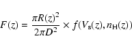 |
(4) |
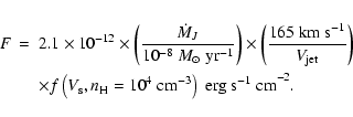
The maximum photocenter displacement will occur at minimum
photospheric brightness. During Hipparcos observations RY Tau V band
magnitudes varied between 9.7 and 11.05. We thus estimate the
continuum flux at minimum brightness in the Hipparcos photometric
filter (
![]() Å) to be
Å) to be
![]() erg s-1 cm-2. The maximum contrast
between line emission from a single shock front and photospheric
continuum emission is therefore expected to be
erg s-1 cm-2. The maximum contrast
between line emission from a single shock front and photospheric
continuum emission is therefore expected to be
![]() for
for
![]() km s-1 and
km s-1 and
![]() for
for
![]() km s-1.
km s-1.
To produce the maximum displacement of the photocenter of 19.5 mas
observed by Hipparcos would thus require a shock front located at a
distance from the star ![]() 300
300
![]() for shock velocities
for shock velocities ![]() 30 km s-1 and 14
30 km s-1 and 14
![]() for shock velocities
for shock velocities
![]() 100 km s-1. But this is well outside the primary beam of
Hipparcos (of diameter 30
100 km s-1. But this is well outside the primary beam of
Hipparcos (of diameter 30
![]() but with a strong
attenuation starting at 5
but with a strong
attenuation starting at 5
![]() from
center). Alternatively, more than one shock front may contribute
within the beam of Hipparcos observations. The photocenter
displacement produced by n shock fronts equally spaced along the jet
within a radius R, i.e. with separations
from
center). Alternatively, more than one shock front may contribute
within the beam of Hipparcos observations. The photocenter
displacement produced by n shock fronts equally spaced along the jet
within a radius R, i.e. with separations
![]() ,
can be
written as:
,
can be
written as:
 |
(5) |
Knot separations ![]() 1
1
![]() are compatible with
previous observations of the inner regions of TTS microjets
(Bacciotti et al. 2000; Dougados et al. 2000; Woitas et al. 2005; López-Martín et al. 2003). Thus
predictions of jet line emission from multiple shocks could
marginally account for the observed Hipparcos photocenter
displacement provided shock velocities are
are compatible with
previous observations of the inner regions of TTS microjets
(Bacciotti et al. 2000; Dougados et al. 2000; Woitas et al. 2005; López-Martín et al. 2003). Thus
predictions of jet line emission from multiple shocks could
marginally account for the observed Hipparcos photocenter
displacement provided shock velocities are ![]() 100 km s-1. This however seems inconsistent with the
non-detection of [N II] emission in RY Tau. Progress on this
issue will require more accurate determinations of shock velocities
through line ratio observations in the RY Tau microjet.
100 km s-1. This however seems inconsistent with the
non-detection of [N II] emission in RY Tau. Progress on this
issue will require more accurate determinations of shock velocities
through line ratio observations in the RY Tau microjet.
Another possible source of photocenter displacement along the jet axis is bright scattered optical light from the surface of the circumstellar disc. At intermediate inclinations for the RY Tau system, the image of the disc in scattered light will be dominated by the blue lobe (see Natta & Whitney 2000 for an example). Occultation of the photosphere will enhance the contrast between scattered and direct stellar light, resulting in a displacement of the photocenter perpendicular to the disc plane, towards the blueshifted jet axis. The maximum degree of linear polarisation of 1.7% at minimum photospheric brightness (Petrov et al. 1999) gives a lower limit to the ratio of scattered to direct light during occultation. Indeed due to polarisation cancelling in a centro-symmetric scattering pattern, the true ratio of scattered to direct light can be much higher than the integrated polarisation. This interpretation should be checked with detailed disc image modelling.
From the fact that the photocenter displacement seen by Hipparcos lies along the jet axis, we thus conclude that a binary companion may not be the most relevant explanation. Our analysis above shows however that line emission from shocks in the jet is probably not bright enough to produce the observed photocenter displacement in the Hipparcos broad photometric filter. The most likely origin thus appears to be scattering off the surface of the disc seen at intermediate inclinations, combined with variable partial occultation of the central photosphere. This interpretation should however be checked with a detailed study of the observed variation of the Hipparcos photocenter with time. In particular, we predict a clear anti-correlation between system brightness and photocenter displacement.
We discuss below whether the transverse velocity shifts marginally
detected at distances along the jet of
![]() 4 and 1
4 and 1
![]() 2 from the star and transverse distances
2 from the star and transverse distances
![]() from the jet axis could be due to rotation within the jet
body. The 2.5
from the jet axis could be due to rotation within the jet
body. The 2.5![]() detection at d//=0
detection at d//=0
![]() 4 is doubtful,
since the inferred sense of rotation would be opposite to the disc
rotation sense inferred from the velocity gradient observed in the
millimetric CO observations of Koerner & Sargent (1995): from blueshifted in
the north-east to redshifted in the south-west along
4 is doubtful,
since the inferred sense of rotation would be opposite to the disc
rotation sense inferred from the velocity gradient observed in the
millimetric CO observations of Koerner & Sargent (1995): from blueshifted in
the north-east to redshifted in the south-west along
![]() .
In contrast, the 3
.
In contrast, the 3![]() detection at
detection at
![]() 2 would indicate a sense of rotation in the jet in
agreement with the disc rotation sense. The detection of jet rotation
at this position and not at others could reflect the fact that both
the SNR and the HVC contribution are maximized there: closer in,
photospheric subtraction residuals are important and the low-velocity
component contributes significantly, while further out, the signal to
noise ratio rapidly decreases. However, interpretation as a rotation
signature remains questionable due to the marginal
2 would indicate a sense of rotation in the jet in
agreement with the disc rotation sense. The detection of jet rotation
at this position and not at others could reflect the fact that both
the SNR and the HVC contribution are maximized there: closer in,
photospheric subtraction residuals are important and the low-velocity
component contributes significantly, while further out, the signal to
noise ratio rapidly decreases. However, interpretation as a rotation
signature remains questionable due to the marginal ![]() level and
to the fact that the detection happens to be very close to the jet
knot detected in the HVB map. We plot in Fig. 5 as white
boxes the two regions of the jet whose summed line profiles produce
the detected transverse velocity shift at 1
level and
to the fact that the detection happens to be very close to the jet
knot detected in the HVB map. We plot in Fig. 5 as white
boxes the two regions of the jet whose summed line profiles produce
the detected transverse velocity shift at 1
![]() 2. The detected
velocity asymmetry could also be caused by asymmetries in the wings of
a bow-shock peaked at the position of the HVB knot, at 1
2. The detected
velocity asymmetry could also be caused by asymmetries in the wings of
a bow-shock peaked at the position of the HVB knot, at 1
![]() 35
from the star (asterisk symbol in the figure). Higher angular
resolution observations that better resolve the jet transverse
structure are required to settle the origin of this velocity
asymmetry.
35
from the star (asterisk symbol in the figure). Higher angular
resolution observations that better resolve the jet transverse
structure are required to settle the origin of this velocity
asymmetry.
We analyze here the derived properties of the RY Tau microjet in the light of previous studies of T Tauri small scale jets. We compare in Fig. 4 the RY Tau blueshifted jet widths as a function of projected distance to the central source with previous studies of TTS microjets. Both the jet widths and opening angle appear similar to those derived on similar spatial scales for the other TTs microjets, suggesting similar collimation scale and properties.
The full range of centroid flow velocities observed on
spatial scales of a few 100 AUs for the DG Tau
(Lavalley et al. 1997; Pyo et al. 2003), RW Aur (Pyo et al. 2006), HL Tau (Pyo et al. 2006),
HH 30 (Hartigan & Morse 2007) and CW Tau (Hartigan et al. 2004) microjets,
where inclination angles are well constrained, is 130-300 km s-1with an average value of
![]() km s-1.
Our possible interval of 100-300 km s-1 for the deprojected
terminal velocity in the RY Tau microjet (Sect. 4.1) thus falls in the same
range as previously investigated microjets from lower mass central
sources.
km s-1.
Our possible interval of 100-300 km s-1 for the deprojected
terminal velocity in the RY Tau microjet (Sect. 4.1) thus falls in the same
range as previously investigated microjets from lower mass central
sources.
Finally, our estimate for the (one-sided) ejection to accretion rate
![]() ratio, between 0.02 and 0.4 with a
best value of 0.085, is also compatible with the average ratio
ratio, between 0.02 and 0.4 with a
best value of 0.085, is also compatible with the average ratio ![]() 0.1 for lower mass cTTS sources found by Cabrit (2007) using
jet mass-fluxes from HEG95 and revised accretion rates from
Gullbring et al. (1998).
0.1 for lower mass cTTS sources found by Cabrit (2007) using
jet mass-fluxes from HEG95 and revised accretion rates from
Gullbring et al. (1998).
The overall properties (collimation, terminal centroid velocities, ejection to accretion rate ratio) of the RY Tau microjet therefore appear quantitatively similar to those of the microjets from lower mass cTTS investigated so far.
The remarkably similar collimation, terminal speed, and ejection efficiency of the RY Tau microjet compared to lower mass cTTs gives for the first time a firm support to the common belief that the jet launching mechanism is probably universal over a broad range of stellar masses. We examine below the implications of the derived RY Tau jet parameters for the three classes of steady state jet launching magneto-centrifugal models currently discussed in the context of cTTS microjets and for which detailed observational predictions are available (see Ferreira et al. 2006; Cabrit 2007, for detailed reviews).
Magnetized stellar wind models have been developped to account for the origin of collimated mass-loss in young stars, and to explain their spin-equilibrium despite active accretion (Sauty & Tsinganos 1994; Matt & Pudritz 2008). Since CTTS rotate at a small fraction of their break-up velocity (e.g. 15% in RY Tau), centrifugal acceleration from the stellar surface is insufficient to overcome the gravitational pull of the star, and a significant amount of energy must be deposited by pressure gradients at the base of the flow. This additional source of energy would presumably originate from the accretion process, e.g. in the form of enthalpy (hot wind) or Alfven-wave pressure (cool wind).
A recent analysis of UV emission lines in RY Tau by
Gómez de Castro & Verdugo (2007) does indicate the presence of
a hot stellar wind at ![]()
![]() K in this star. However,
with the parameters derived by these authors for the UV line emitting region (emitting
volume (0.35
K in this star. However,
with the parameters derived by these authors for the UV line emitting region (emitting
volume (0.35 ![]() )3, total density
)3, total density ![]() 1010 cm-3 and flow velocity
1010 cm-3 and flow velocity ![]() 150 km s-1), we
estimate a mass-loss rate for the high-temperature UV emitting wind of
150 km s-1), we
estimate a mass-loss rate for the high-temperature UV emitting wind of ![]()
![]() yr-1. This is 2-3 orders of magnitude
lower than the mass-loss rate in the optical jet. Thus,
the hot stellar wind component does not contribute significantly to the
bulk of the jet mass-loss seen at optical wavelengths, and
enthalpy is not the main jet driving mechanism.
yr-1. This is 2-3 orders of magnitude
lower than the mass-loss rate in the optical jet. Thus,
the hot stellar wind component does not contribute significantly to the
bulk of the jet mass-loss seen at optical wavelengths, and
enthalpy is not the main jet driving mechanism.
Pressure gradients from Alfvén waves allow one to drive cooler stellar
winds (Decampli 1981), but the wave energy needed to power the
observed jet mass flux is unrealistically large. Neglecting centrifugal
acceleration, the fraction of accretion luminosity that needs to be
transferred to the flow is
![]() where
where
![]() is the mass-flux in one
jet and
is the mass-flux in one
jet and
![]() parametrizes the
amount of specific energy transferred to the flow by pressure
gradients (Ferreira et al. 2006). In RY Tau, the estimated range of jet
terminal speed is 100-300 km s-1 and the Keplerian speed at the
stellar surface
parametrizes the
amount of specific energy transferred to the flow by pressure
gradients (Ferreira et al. 2006). In RY Tau, the estimated range of jet
terminal speed is 100-300 km s-1 and the Keplerian speed at the
stellar surface
![]() 350 km s-1(using
350 km s-1(using
![]() and
and
![]() ;
Calvet et al. 2004), yielding
;
Calvet et al. 2004), yielding
![]() and
and
![]() for the one-sided
ejection/accretion ratio of 0.1. Full MHD stellar wind solutions
including magnetocentrifugal effects yield a similar result, with
for the one-sided
ejection/accretion ratio of 0.1. Full MHD stellar wind solutions
including magnetocentrifugal effects yield a similar result, with
![]() % for a two-sided ejection/accretion
ratio of
0.15-0.2 (Matt & Pudritz 2008). If only 20% of the Alfvén wave
power is actually transferred to the flow, as the calculations of
Decampli (1981) suggest, the total power in waves would have to be
comparable to the accretion luminosity, which seems unrealistic.
% for a two-sided ejection/accretion
ratio of
0.15-0.2 (Matt & Pudritz 2008). If only 20% of the Alfvén wave
power is actually transferred to the flow, as the calculations of
Decampli (1981) suggest, the total power in waves would have to be
comparable to the accretion luminosity, which seems unrealistic.
We now examine the possibility that the jet originates from the inner
regions of the circumstellar disc (X-wind or extended disc wind). The
expression of the terminal poloidal flow velocity for a given
streamline originating from a launching radius r0 in the disc is
given by (Blandford & Payne 1982):
 |
(6) |
In the framework of the X-wind model developed by Shu and
collaborators, all the streamlines originate from the co-rotation
radius in the disc with ![]() values ranging between 3 and 6
(Shang et al. 1998), with most of the mass flux having
values ranging between 3 and 6
(Shang et al. 1998), with most of the mass flux having
![]() .
With the RY Tau stellar parameters
.
With the RY Tau stellar parameters
![]() ,
,
![]() ,
and
,
and ![]() = 52 km s-1, we estimate a co-rotation
radius of
= 52 km s-1, we estimate a co-rotation
radius of
![]() AU. Thus, the range of terminal poloidal
velocities predicted by the X-wind model in the case of the RY Tau
microjet would be
AU. Thus, the range of terminal poloidal
velocities predicted by the X-wind model in the case of the RY Tau
microjet would be ![]()
![]() km s-1, with the jet
line emission sharply peaked at the lower value (see predicted PV
diagrams in Shang et al. 1998). The [O I] velocity centroid of 70 km s-1 in the RY Tau jet would then imply an inclination of
the jet axis to the line of sight of 77
km s-1, with the jet
line emission sharply peaked at the lower value (see predicted PV
diagrams in Shang et al. 1998). The [O I] velocity centroid of 70 km s-1 in the RY Tau jet would then imply an inclination of
the jet axis to the line of sight of 77![]() ,
at the upper limit
of current observational constraints (see Sect. 4.1).
,
at the upper limit
of current observational constraints (see Sect. 4.1).
In the radially self-similar disc wind solutions first introduced by
Blandford & Payne (1982), mass-loss originates from an extended range of radii in
the disc, and the magnetic lever arm parameter ![]() is constant
over all streamlines. Self-consistent calculations including the accretion disk
dynamics show that super-Alfvénic solutions exist for
is constant
over all streamlines. Self-consistent calculations including the accretion disk
dynamics show that super-Alfvénic solutions exist for
![]() between 2 and 100, depending on the toroidal field and
heating at the disk surface (Casse & Ferreira 2000; Ferreira 1997). The
two-sided ejection to accretion rate ratio is tightly related to
between 2 and 100, depending on the toroidal field and
heating at the disk surface (Casse & Ferreira 2000; Ferreira 1997). The
two-sided ejection to accretion rate ratio is tightly related to
![]() and is given by
and is given by
![]() where
where
![]() and
and
![]() are the inner
and outer radii of the region in the disc where the jet originates. As
shown in Ferreira et al. (2006), these solutions reproduce the global
properties (collimation, terminal poloidal velocities, rotation
signatures, ejection to accretion rate ratio) of previously studied
cTTs microjets for
are the inner
and outer radii of the region in the disc where the jet originates. As
shown in Ferreira et al. (2006), these solutions reproduce the global
properties (collimation, terminal poloidal velocities, rotation
signatures, ejection to accretion rate ratio) of previously studied
cTTs microjets for ![]() values in the range 2-15 and
values in the range 2-15 and
![]() a few AUs. The global derived RY Tau jet parameters, being in the
same range as previously investigated cTTS microjets, will therefore
be compatible with similar disc wind solutions. We note in particular
that the transverse kinematical structure of the blueshifted jet,
illustrated in Fig. 7, is reminiscent of the
kinematical behavior of magneto-centrifugal disc winds where outer
streamlines originating from larger launching radii are predicted to
flow at lower velocities than inner streamlines.
a few AUs. The global derived RY Tau jet parameters, being in the
same range as previously investigated cTTS microjets, will therefore
be compatible with similar disc wind solutions. We note in particular
that the transverse kinematical structure of the blueshifted jet,
illustrated in Fig. 7, is reminiscent of the
kinematical behavior of magneto-centrifugal disc winds where outer
streamlines originating from larger launching radii are predicted to
flow at lower velocities than inner streamlines.
Our current best estimates of the RY Tau microjet parameters thus appear more compatible with an origin from the inner regions of the disc than with a stellar wind. Obviously, an accurate determination of the jet parameters (inclination and densities) is required to constrain more precisely the wind kinematics and the ejection to accretion ratio, allowing a detailed comparison with model predictions.
Using the OASIS spectroimager at CFHT, we have studied with 0.2
![]() -0.4
-0.4
![]() resolution the 2D morphology and kinematics of the inner
2
resolution the 2D morphology and kinematics of the inner
2
![]() of the RY Tau microjet in the [O I]
of the RY Tau microjet in the [O I]![]() 6300 Å line. Our main conclusions are the following:
6300 Å line. Our main conclusions are the following:
Acknowledgements
We are grateful to the anonymous referee for useful and constructive comments. V. Agra-Amboage, S. Cabrit, and P. Garcia wish to acknowledge financial and travel support through the Marie Curie Research Training Network JETSET (Jet Simulations, Experiments and Theory) under contract MRTN-CT-2004-005592. The work of P. Garcia was supported in part by the Fundação para a Ciencia e a Tecnologia through grant PTDC/CTEAST/65971/2006 from POTCI, with funds from the European program FEDER.
In order to accurately estimate the uncertainties due to noise in our
transverse velocity shift measurements, we perform a Monte-Carlo study adapted
to our OASIS observational parameters.
We simulate pairs of identical
Gaussian spectra with total FWHM 135 km s-1 or 175 km s-1,
typical of our observations, and shift them by
![]() km s-1 (comparable to the expected transverse velocity shifts due to
rotation), using the same velocity sampling as in our data. We
checked that the results shown below are in fact independent of the
shift for
km s-1 (comparable to the expected transverse velocity shifts due to
rotation), using the same velocity sampling as in our data. We
checked that the results shown below are in fact independent of the
shift for
![]() km s-1. We then introduce random Gaussian
noise typical of our observing parameters, i.e. a peak signal-to-noise
ratio (SNR) varying between 5 and 40. For each Monte-Carlo realisation of
the noise statistics, we ``measure'' velocity shifts between the two
spectra with the two different methods: difference between the
velocity centroids derived from single component Gaussian fits, and
cross-correlation between the pair of spectra. We perform 300 such
Monte-Carlo realisations at a given SNR, and then compute the rms
standard deviation of the 300 measured velocity shifts.
km s-1. We then introduce random Gaussian
noise typical of our observing parameters, i.e. a peak signal-to-noise
ratio (SNR) varying between 5 and 40. For each Monte-Carlo realisation of
the noise statistics, we ``measure'' velocity shifts between the two
spectra with the two different methods: difference between the
velocity centroids derived from single component Gaussian fits, and
cross-correlation between the pair of spectra. We perform 300 such
Monte-Carlo realisations at a given SNR, and then compute the rms
standard deviation of the 300 measured velocity shifts.
The result is shown in Fig. A.1 where we plot the standard deviation of the measured velocity shift as a function of initial peak signal to noise ratio for the 2 methods, and for the two values of input FWHM. This study demonstrates that the Gaussian fitting procedure gives the best accuracy compared to cross-correlation, and that the error increases steeply with decreasing peak SNR.
The theoretical accuracy on the centroid of a single component
Gaussian profile of dispersion
![]() dominated by photon
noise and with infinite sampling is given by
dominated by photon
noise and with infinite sampling is given by
![]() /SNR
(Porter et al. 2004) where the SNR is the signal over noise ratio at the line
emission peak. Since we compute the difference of two centroids, each
affected by the same error, we would thus expect a 1
/SNR
(Porter et al. 2004) where the SNR is the signal over noise ratio at the line
emission peak. Since we compute the difference of two centroids, each
affected by the same error, we would thus expect a 1![]() dispersion in the velocity shifts of
dispersion in the velocity shifts of
![]() ranging between
ranging between
![]() km s-1 (for
km s-1 (for
![]() km s-1) and
km s-1) and
![]() km s-1 (for
km s-1 (for
![]() km s-1). Our Monte-Carlo results in
Fig. A.1 for the Gaussian method are well fitted by an
empirical formula
km s-1). Our Monte-Carlo results in
Fig. A.1 for the Gaussian method are well fitted by an
empirical formula
![]() km s-1,
fully consistent with the theoretical expectations from
Porter et al. (2004). We use this formula to compute
3
km s-1,
fully consistent with the theoretical expectations from
Porter et al. (2004). We use this formula to compute
3![]() error bars for the transverse velocity shifts
plotted in Fig. 8.
error bars for the transverse velocity shifts
plotted in Fig. 8.
![\begin{figure}
\par\includegraphics[width=8.4cm,clip]{0025fgA1.ps}
\end{figure}](/articles/aa/full/2009/03/aa10025-08/img213.gif) |
Figure A.1:
1 |
| Open with DEXTER | |