A&A 493, 331-337 (2009)
DOI: 10.1051/0004-6361:200811040
Reducing the gravitational lensing scatter of type Ia supernovae without introducing any extra bias
J. Jönsson1 - E. Mörtsell2 - J. Sollerman3,4
1 - University of Oxford Astrophysics, Denys Wilkinson
Building, Keble Road, Oxford OX1 3RH, UK
2 -
Physics Department, Stockholm University, AlbaNova University Center, 10691
Stockholm, Sweden
3 -
Stockholm Observatory, AlbaNova, Department of Astronomy, 10691
Stockholm, Sweden
4 -
Dark Cosmology Centre, Niels Bohr
Institute, University of Copenhagen, Juliane Maries Vej 30, 2100
Copenhagen Ø, Denmark
Received 25 September 2008 / Accepted 14 October 2008
Abstract
Aims. Magnification and de-magnification due to gravitational lensing will contribute to the brightness scatter of type Ia supernovae (SNe Ia). The purpose of this paper is to investigate the possibility of decreasing this scatter by correcting individual SNe Ia using observations of galaxies in the foreground, without introducing any extra bias.
Methods. We simulate a large number of SN Ia lines of sight populated by galaxies. For each line of sight the true magnification factor and an estimate thereof are calculated. The estimated magnification factor corresponds to what an observer would infer from a survey like the SNLS. Using the simulated data we investigate the possibility of estimating the magnification of individual supernovae with enough precision to be able to correct their brightness for gravitational lensing with negligible bias.
Results. Our simulations show that the bias arising from gravitational lensing corrections of individual SNe Ia is negligible for current and next generation surveys and that the scatter from lensing can be reduced by approximately a factor of 2. The total scatter in the SN Ia magnitudes could be reduced by  for an intrinsic dispersion of 0.13 mag. For an intrinsic dispersion of 0.09 mag, which may be feasible for future surveys, the total scatter could be reduced by
  .
This will reduce the errors on cosmological parameters derived from supernova data by 4-8%. The prospect of correcting for lensing is thus very good.
.
This will reduce the errors on cosmological parameters derived from supernova data by 4-8%. The prospect of correcting for lensing is thus very good.
Key words: star: supernovae: general - gravitational lensing - cosmology: large-scale structure of Universe - cosmology: cosmological parameters - cosmology: observations
Large dedicated supernova surveys, such
as SNLS (Astier et al. 2006),
ESSENCE (Wood-Vasey et al. 2007; Miknaitis et al. 2007), and
SDSS-II (Frieman et al. 2008),
have gathered data on a large number
of supernovae at cosmological redshifts.
Consequently, supernova
cosmology has now reached a stage where systematic uncertainties,
rather than lack of statistics, limit the ability to constrain
cosmological models.
Extinction by dust and peculiar motions of host galaxies seem to
be the systematic effects which currently pose the largest
difficulties (e.g. Leibundgut 2008). In this paper we investigate the
possibility of correcting for
another systematic uncertainty - gravitational lensing.
In an inhomogeneous universe like ours, light from
a distant type Ia supernova (hereafter SN Ia) is inevitably
affected by gravitational lensing. Weak gravitational lensing,
which is what we will consider in this paper, refers to
the phenomena which occur when a bundle of light rays is
distorted by the gravitational fields exerted by matter. The distortion
can lead to magnification or de-magnification of the SN Ia flux.
This (de)magnification
can be described by the magnification factor,  ,
which depends on
the distribution and composition of the foreground matter.
Both baryonic and dark matter influence the trajectories of photons, but
since the latter dominates on the scales relevant for this work,
we only use the baryonic
component as a tracer of the dark matter.
If an observer residing in a homogeneous universe would measure the flux f,
an observer situated in an inhomogeneous universe will measure the flux
,
which depends on
the distribution and composition of the foreground matter.
Both baryonic and dark matter influence the trajectories of photons, but
since the latter dominates on the scales relevant for this work,
we only use the baryonic
component as a tracer of the dark matter.
If an observer residing in a homogeneous universe would measure the flux f,
an observer situated in an inhomogeneous universe will measure the flux
 .
Due to flux conservation, as long as we do not have multiple images,
the probability distribution function for the magnification
factor,
.
Due to flux conservation, as long as we do not have multiple images,
the probability distribution function for the magnification
factor,  ,
satisfies the constraint
,
satisfies the constraint
 ,
i.e. the average magnification factor is unity.
The effect of gravitational lensing consequently averages out, which
implies that
this systematic effect can be controlled by observing large numbers of SNe Ia.
In reality however,
,
i.e. the average magnification factor is unity.
The effect of gravitational lensing consequently averages out, which
implies that
this systematic effect can be controlled by observing large numbers of SNe Ia.
In reality however,
 converges very slowly towards unity as the
sample size increases (Holz & Linder 2005). This is due to the fact that the whole distribution
of ,
including its elusive high magnification tail, must be sampled,
which in addition to large numbers also requires large survey areas (Cooray et al. 2006).
converges very slowly towards unity as the
sample size increases (Holz & Linder 2005). This is due to the fact that the whole distribution
of ,
including its elusive high magnification tail, must be sampled,
which in addition to large numbers also requires large survey areas (Cooray et al. 2006).
Although the bias in principle can be decreased by large numbers,
gravitational lensing still contributes to the
brightness scatter of SNe Ia.
This contribution increases with
redshift and is expected to be substantial at  (Holz & Linder 2005).
For precision measurements of cosmological parameters it is therefore desirable
to minimize this scatter by measuring and correcting for the
gravitational lensing effect.
(Holz & Linder 2005).
For precision measurements of cosmological parameters it is therefore desirable
to minimize this scatter by measuring and correcting for the
gravitational lensing effect.
The method we rely upon is based on modeling the dark matter haloes, which
surround galaxies, using the observed properties of the galaxies. This method
takes into account contributions to the lensing from sub-arc-minute scales, which makes
it a viable method, in contrast to shear maps (Dalal et al. 2003) which are insensitive to these scales.
The possibility of correcting individual SNe Ia for gravitational lensing
using the method considered here
was investigated by Gunnarsson et al. (2006), where simulations showed that the
lensing scatter could be reduced by almost a factor of 3 for a source at
redshift z=1.5. In this paper we focus on the possibility of correcting
for gravitational lensing at the lower redshifts ( )
accessible to the aforementioned large ground based surveys.
The simulations aim at mimicking the supernova legacy survey (SNLS, Astier et al. 2006), and follow
closely the strategy by Jönsson et al. (2008, hereafter J08).
)
accessible to the aforementioned large ground based surveys.
The simulations aim at mimicking the supernova legacy survey (SNLS, Astier et al. 2006), and follow
closely the strategy by Jönsson et al. (2008, hereafter J08).
For a correction to be
useful the following two criteria must be met:
- 1.
- the correction should decrease the scatter in SN Ia magnitudes due to gravitational
lensing;
- 2.
- any bias introduced in the SN Ia magnitudes from the correction should be negligible.
In Sect. 2, we use simulated data to
investigate the possibility of performing corrections satisfying the
two criteria above.
The method we use to correct for lensing
is explained and applied to the simulated data in Sect. 3.
Our results are discussed and summarized in
Sect. 4.
2 Simulations
Since our simulations are very similar to the ones presented in
more detail by J08, we only provide a brief presentation here.
We have simulated deep galaxy catalogs with properties
(galaxy positions, redshifts, luminosities, types)
based on real observations (Dahlén et al. 2005). For a single line of sight we first
compute the true magnification factor,
 ,
using the multiple lens plane algorithm implemented in the Q-LET package (Gunnarsson 2004). All galaxies are
included in the calculation and the dark matter haloes surrounding each
galaxy are modeled by truncated Navarro-Frenk-White (NFW, Navarro et al. 1997) profiles.
Then we compute the magnification factor which an observer
(with access to SNLS data) would estimate,
,
using the multiple lens plane algorithm implemented in the Q-LET package (Gunnarsson 2004). All galaxies are
included in the calculation and the dark matter haloes surrounding each
galaxy are modeled by truncated Navarro-Frenk-White (NFW, Navarro et al. 1997) profiles.
Then we compute the magnification factor which an observer
(with access to SNLS data) would estimate,
 ,
for the same line of sight. The observer would, for example, only see galaxies brighter
than the magnitude limit (
,
for the same line of sight. The observer would, for example, only see galaxies brighter
than the magnitude limit (
 )
of the survey and would probably have access only to
photometric redshifts (with a precision of
)
of the survey and would probably have access only to
photometric redshifts (with a precision of
 for most galaxies, but failing catastrophically for 2-6% of the galaxies).
The content of the line of sight is therefore rather different
when the true and estimated magnifications are calculated.
Since the observer does not know what the correct model is,
there is also a difference in the model used to compute the true and the estimated
magnification factor.
Since the effects of gravitational lensing are redshift dependent, we
simulate gravitational lensing of sources in the redshift range
for most galaxies, but failing catastrophically for 2-6% of the galaxies).
The content of the line of sight is therefore rather different
when the true and estimated magnifications are calculated.
Since the observer does not know what the correct model is,
there is also a difference in the model used to compute the true and the estimated
magnification factor.
Since the effects of gravitational lensing are redshift dependent, we
simulate gravitational lensing of sources in the redshift range
 ,
relevant for e.g. the SNLS survey.
,
relevant for e.g. the SNLS survey.
The result of the simulations are hence pairs of true,
,
and
estimated,
,
magnification factors.
Since most cosmology fits to date have been performed
using magnitudes rather than fluxes, we treat magnification in terms
of logarithmic units. Throughout the paper we denote true and
estimated magnifications by
 and
and
 ,
respectively.
,
respectively.
Figure 1 shows
simulated pairs of magnification factors in logarithmic units.
This plot shows most of the simulated pairs, but not the
small fraction (
 )
belonging
to the high magnification tail with
)
belonging
to the high magnification tail with
 .
The scatter in this plot comes mostly from
the uncertainty in the model used to
convert galaxy luminosity to mass (in our case Tully-Fisher and Faber-Jackson relations).
Given the importance of the luminosity-to-mass
model, we continue this investigation by considering
three different scenarios, all shown in Fig. 1:
.
The scatter in this plot comes mostly from
the uncertainty in the model used to
convert galaxy luminosity to mass (in our case Tully-Fisher and Faber-Jackson relations).
Given the importance of the luminosity-to-mass
model, we continue this investigation by considering
three different scenarios, all shown in Fig. 1:
- 1.
- no shift in halo masses (circles);
- 2.
- underestimated halo masses (squares);
- 3.
- overestimated halo masses (triangles).
If the masses of the dark matter haloes are substantially overestimated
(by 50 in scenario 2) or underestimated (by 50
in scenario 3),
the gravitational magnification estimates will be erroneous.
Our simulations aim to investigate to what
extent a proper correction can be made for the lensing magnification given these uncertainties.
Other sources of uncertainty, such as scatter in
the luminosity-to-mass model, were also included for all three scenarios.
Clearly, the distributions
of points in the plot differ for the three scenarios.
True and estimated magnification factors are apparently correlated in
all scenarios, albeit with different slopes. The no shift scenario has a slope
(outlined by the solid line in Fig. 1)
near unity, which
reflects the fact that the model used to estimate the magnification is
very close to the correct one. The underestimation (dashed line) and
overestimation (dotted line) scenarios have slopes which differ from unity.
in scenario 2) or underestimated (by 50
in scenario 3),
the gravitational magnification estimates will be erroneous.
Our simulations aim to investigate to what
extent a proper correction can be made for the lensing magnification given these uncertainties.
Other sources of uncertainty, such as scatter in
the luminosity-to-mass model, were also included for all three scenarios.
Clearly, the distributions
of points in the plot differ for the three scenarios.
True and estimated magnification factors are apparently correlated in
all scenarios, albeit with different slopes. The no shift scenario has a slope
(outlined by the solid line in Fig. 1)
near unity, which
reflects the fact that the model used to estimate the magnification is
very close to the correct one. The underestimation (dashed line) and
overestimation (dotted line) scenarios have slopes which differ from unity.
From Fig. 1, the asymmetry of both the distribution of
 and
and
 is evident.
For
slopes differing from unity this asymmetry implies an asymmetry in
the errors in the estimated magnifications.
The estimated magnification of a SN Ia in the high
magnification tail (negative values in Fig. 1) is likely to
be more erroneous than a typical SN Ia which is slightly de-magnified
(positive values in Fig. 1).
is evident.
For
slopes differing from unity this asymmetry implies an asymmetry in
the errors in the estimated magnifications.
The estimated magnification of a SN Ia in the high
magnification tail (negative values in Fig. 1) is likely to
be more erroneous than a typical SN Ia which is slightly de-magnified
(positive values in Fig. 1).
![\begin{figure}
\resizebox{9cm}{!}{\includegraphics[angle=-90]{1040fig1.eps}}
\end{figure}](/articles/aa/full/2009/01/aa11040-08/Timg34.gif) |
Figure 1:
True magnification,
,
versus estimated magnification,
,
for three different scenarios: no shift in halo masses (circles),
underestimated halo masses (squares), and
overestimated halo masses (triangles).
The straight lines show the best fits
to the no shift (solid line), underestimation (dashed line), and
overestimation (dotted line) scenario. |
| Open with DEXTER |
3 Gravitational lensing corrections
Since gravitationally magnified (de-magnified) SNe Ia should be
brighter (fainter) than the average supernova, a correlation between
estimated magnification and SN Ia brightness is expected.
According to Fig. 1, which can be seen as an idealized
magnification-residual diagram, a correlation
is expected even if the model used to estimate the magnification
factors is biased.
A real magnification-residual diagram,
where Hubble diagram residuals are used instead of
,
will also be smeared by, e.g., measurement errors and
intrinsic brightness scatter.
We take the supernova Hubble diagram residuals
to be the differences between observed magnitudes,
 ,
and
magnitudes predicted by a cosmological model
of a homogeneous universe (we assume a flat universe, dominated
by a cosmological constant, with
,
and
magnitudes predicted by a cosmological model
of a homogeneous universe (we assume a flat universe, dominated
by a cosmological constant, with
 and
H0=70 km s-1 Mpc-1).
In the following, we assume that the residuals have been
computed using the correct cosmological model. The residual is then
the sum of
and noise,
and
H0=70 km s-1 Mpc-1).
In the following, we assume that the residuals have been
computed using the correct cosmological model. The residual is then
the sum of
and noise,
 ,
from,
e.g., intrinsic SN Ia
brightness scatter and measurement errors. We ignore other
systematic sources of uncertainty and assume the noise to be Gaussian.
,
from,
e.g., intrinsic SN Ia
brightness scatter and measurement errors. We ignore other
systematic sources of uncertainty and assume the noise to be Gaussian.
Because of gravitational lensing, an observer in an inhomogeneous universe
measures the magnitude
 |
(1) |
rather than the magnitude
 ,
which would
be measured if the observer resided in a homogeneous universe.
The effect of gravitational lensing averages out because the average
magnification factor is unity.
However, an infinite number of SNe Ia is in principle
required, since
the average magnification factor
of a finite sample converges very slowly to unity as the sample size increases
(see Fig. 2 in Holz & Linder 2005).
When magnitudes are used instead of fluxes, on the other hand, the effect no
longer averages out even in principle, because
,
which would
be measured if the observer resided in a homogeneous universe.
The effect of gravitational lensing averages out because the average
magnification factor is unity.
However, an infinite number of SNe Ia is in principle
required, since
the average magnification factor
of a finite sample converges very slowly to unity as the sample size increases
(see Fig. 2 in Holz & Linder 2005).
When magnitudes are used instead of fluxes, on the other hand, the effect no
longer averages out even in principle, because
 even though
 .
Observed magnitudes are consequently
biased by an amount depending on the redshift.
The thick solid curve in
Fig. 2a shows this bias,
.
Observed magnitudes are consequently
biased by an amount depending on the redshift.
The thick solid curve in
Fig. 2a shows this bias,
 ,
which
is of the order 10-3.
,
which
is of the order 10-3.
Recently Sarkar et al. (2008) investigated the expected bias
in the dark energy equation of state parameter
due to gravitational lensing for
future SN Ia surveys. In their study Sarkar et al. (2008) considered both
averaging over magnitudes (as we do here) and a flux-averaging
technique (Wang & Mukherjee 2004; Wang 2000). In both cases they found the resulting
bias in the equation of state parameter to be negligible, compared to the
expected statistical uncertainty.
![\begin{figure}
\resizebox{9cm}{!}{\includegraphics[angle=-90]{1040fig2.eps}}
\end{figure}](/articles/aa/full/2009/01/aa11040-08/Timg43.gif) |
Figure 2:
Bias (panel a)) and dispersion (panel b))
in  as a function of redshift.
The no shift scenario is represented by
the thin solid curves. Dashed and dotted curves correspond
to the under- and overestimation scenarios, respectively.
Bias and dispersion of
,
outlined by the thick solid curves, are also shown for comparison. The
estimated magnifications,
,
were used to correct for gravitational
lensing.
as a function of redshift.
The no shift scenario is represented by
the thin solid curves. Dashed and dotted curves correspond
to the under- and overestimation scenarios, respectively.
Bias and dispersion of
,
outlined by the thick solid curves, are also shown for comparison. The
estimated magnifications,
,
were used to correct for gravitational
lensing. |
| Open with DEXTER |
3.3 Lensing corrections
If the estimated magnification factors are used to correct
for gravitational lensing, the corrected magnitudes would be
 |
(2) |
where the correction is characterized by the difference
 |
(3) |
For the correction to be useful, according to the first criterion stated
above, the dispersion in the SN Ia magnitudes must be decreased
(
 ), which
consequently means that
the dispersion in
must be smaller than the dispersion in
,
i.e.
), which
consequently means that
the dispersion in
must be smaller than the dispersion in
,
i.e.
 .
.
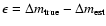
The second criterion requires that the correction does not introduce
any extra bias in the corrected magnitudes. According to
Eq. (2) this bias is given by
 .
Whether the bias is negligible or not depends on the
size of the statistical error. We require
.
Whether the bias is negligible or not depends on the
size of the statistical error. We require
 for a correction to be considered useful.
Figures 2a and b show the bias and
dispersion, respectively,
for
computed for the three different scenarios
discussed in Sect. 2 over a range
of redshifts. In this case, no noise has been taken into account.
The scenario corresponding to no shift in halo mass is shown by the thin solid curves.
Thin dashed and dotted curves outline the results for
the scenarios were halo masses have been under- and overestimated,
respectively.
We also display with the thick solid curves the bias and dispersion in
.
For all three scenarios, the first criterion above is fulfilled,
i.e.
 at all redshifts.
At
at all redshifts.
At
 ,
which is the redshift where the SNLS distribution of SNe Ia peaks,
the reduction in the scatter is a factor 2.1, 1.9, and 1.8 for scenario 1, 2, and 3.
The absolute value of the bias,
,
which is the redshift where the SNLS distribution of SNe Ia peaks,
the reduction in the scatter is a factor 2.1, 1.9, and 1.8 for scenario 1, 2, and 3.
The absolute value of the bias,
 ,
is
,
is
 for all scenarios. If this
bias is divided by
for all scenarios. If this
bias is divided by
 ,
we find
,
we find
 ,
which
implies successful corrections for all cases and at all redshifts
according to our second criterion.
Moreover, for all three scenarios
,
which
implies successful corrections for all cases and at all redshifts
according to our second criterion.
Moreover, for all three scenarios
 .
We have thereby demonstrated that such a correction for
gravitational lensing would clearly decrease the scatter in the
Hubble diagram without adding significant bias after the corrections.
.
We have thereby demonstrated that such a correction for
gravitational lensing would clearly decrease the scatter in the
Hubble diagram without adding significant bias after the corrections.
Let us now investigate the potential
benefits of gravitational lensing corrections in
the presence of realistic intrinsic brightness scatter and measurement errors.
We have simulated SNLS-like data sets, consisting of 250 SNe Ia each,
for the three scenarios.
Since the results depend on the assumed errors, we have also varied the
intrinsic brightness scatter in the simulations. To model the measurement errors
we have used the following fit to the first year SNLS data (Astier et al. 2006):
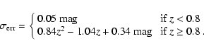 |
(4) |
For each simulated data set,
,
 ,
and
were computed.
Figure 3 shows scatter plots of
,
and
were computed.
Figure 3 shows scatter plots of
 (the second criterion)
versus
(the second criterion)
versus
 (the first criterion)
for different assumed errors.
As in Fig. 1 the three scenarios are indicated by different plotting symbols.
In Fig. 3a measurement errors, modeled by Eq. (4), and intrinsic dispersion,
(the first criterion)
for different assumed errors.
As in Fig. 1 the three scenarios are indicated by different plotting symbols.
In Fig. 3a measurement errors, modeled by Eq. (4), and intrinsic dispersion,
 mag, correspond to the precision of first year SNLS data. A future decrease
in the intrinsic dispersion is possible. We therefore show in Fig. 3b results obtained
for the same measurement errors, but with
mag, correspond to the precision of first year SNLS data. A future decrease
in the intrinsic dispersion is possible. We therefore show in Fig. 3b results obtained
for the same measurement errors, but with
 mag. Figure 3c shows
results for
mag and negligible measurement errors, i.e.
mag. Figure 3c shows
results for
mag and negligible measurement errors, i.e.
 mag.
For comparison we also show results in Fig. 3d for an intrinsic dispersion of only
0.05 mag and
mag.
The distributions of points
in the scatter plots are rather similar irrespective of the scenario.
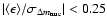
A value of
less than unity, i.e. to the left of the vertical lines,
indicates a successful correction according to the first criterion.
The number of simulated data sets failing to meet the first criterion,
i.e. points to the right of the vertical line, decreases as
the errors decrease. In Fig. 3a the
correction fails for 4%, 1%, and 10% of the synthetic data sets
for the no shift, underestimation, and overestimation scenario. These numbers
drop to less than one percent for Fig. 3d.
mag.
For comparison we also show results in Fig. 3d for an intrinsic dispersion of only
0.05 mag and
mag.
The distributions of points
in the scatter plots are rather similar irrespective of the scenario.
A value of
less than unity, i.e. to the left of the vertical lines,
indicates a successful correction according to the first criterion.
The number of simulated data sets failing to meet the first criterion,
i.e. points to the right of the vertical line, decreases as
the errors decrease. In Fig. 3a the
correction fails for 4%, 1%, and 10% of the synthetic data sets
for the no shift, underestimation, and overestimation scenario. These numbers
drop to less than one percent for Fig. 3d.
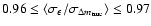
From Fig. 3 it is also evident that the bias after the correction
has been performed is small; for all cases
 .
According to Fig. 3, corrections for gravitational lensing are likely
to reduce the scatter in SN Ia brightness without introducing any harmful bias.
.
According to Fig. 3, corrections for gravitational lensing are likely
to reduce the scatter in SN Ia brightness without introducing any harmful bias.
![\begin{figure}
\resizebox{9cm}{!}{\includegraphics[angle=-90]{1040fig3.eps}}
\end{figure}](/articles/aa/full/2009/01/aa11040-08/Timg61.gif) |
Figure 3:
Scatter plot of
versus
for simulated SNLS-like data sets
consisting of 250 SNe Ia each.
Circles, squares, and triangles represent the no shift, under-, and overestimation
scenarios, respectively.
The different panels correspond to different
intrinsic brightness dispersion and measurement errors:
panel a)
mag,
 given by Eq. (4);
panel b)
mag,
given by Eq. (4);
panel c)
mag,
mag;
panel d)
given by Eq. (4);
panel b)
mag,
given by Eq. (4);
panel c)
mag,
mag;
panel d)
 mag,
mag.
mag,
mag. |
| Open with DEXTER |
Figure 4 shows a projection of Fig. 3
focusing on the distribution of the ratio
.
Figures 4a-c show results
obtained for the no shift, under-, and overestimation scenarios.
Solid and dashed curves correspond to measurement errors modeled
by Eq. (4) and an intrinsic dispersion of 0.13 and 0.09 mag, respectively.
Dotted and dash-dotted curves correspond to negligible measurement errors
(
mag) and intrinsic dispersions of 0.09 and 0.05 mag, respectively.
In Table 1, the characteristics of the distributions
shown in Fig. 4 are summarized.
From Fig. 4,
it is clear that the distributions obtained
with systematic shifts in the halo masses (scenario 2 and 3) are similar to the
distributions corresponding to the no shift scenario.
From Table 1 we see that
 when the intrinsic scatter is
mag,
which implies that the average effect of correcting for gravitational
lensing is to decrease the total scatter by 3-4%.
A realistic future intrinsic dispersion of
mag would allow
a decrease in the total scatter by 5-6%, for measurement errors modeled by
Eq. (4), and by 7-8% if measurement errors could be reduced to a negligible level.
when the intrinsic scatter is
mag,
which implies that the average effect of correcting for gravitational
lensing is to decrease the total scatter by 3-4%.
A realistic future intrinsic dispersion of
mag would allow
a decrease in the total scatter by 5-6%, for measurement errors modeled by
Eq. (4), and by 7-8% if measurement errors could be reduced to a negligible level.
We have also investigated the possible improvements on cosmological
parameter estimation that could be gained from
gravitational lensing corrections.
Using the Fisher information matrix, we computed confidence ellipses in the
 -plane assuming a flat universe. The parameters
 and w denote the dimensionless matter density of the universe and
a constant dark energy equation of state parameter, respectively. In this analysis,
a low and a high redshift SN Ia data set were used. The high redshift data set
consists of 250 SNe Ia with redshifts and measurements errors similar to
first year SNLS data (Astier et al. 2006). The purpose of the low redshift data set, consisting of
44 SNe Ia unaffected by lensing, is to anchor the Hubble diagram.
Redshifts and uncertainties were similar to the low redshift data set used in Astier et al. (2006).
Errors due to gravitational lensing before and after correction were modeled using
the curves in Fig. 2. Our treatment of the errors is hence simplified, because these curves
correspond to the dispersion and do not take the asymmetry of the distributions into account.
Table 2 shows the
relative improvement in the area of the confidence level ellipses due to gravitational
lensing corrections,
and w denote the dimensionless matter density of the universe and
a constant dark energy equation of state parameter, respectively. In this analysis,
a low and a high redshift SN Ia data set were used. The high redshift data set
consists of 250 SNe Ia with redshifts and measurements errors similar to
first year SNLS data (Astier et al. 2006). The purpose of the low redshift data set, consisting of
44 SNe Ia unaffected by lensing, is to anchor the Hubble diagram.
Redshifts and uncertainties were similar to the low redshift data set used in Astier et al. (2006).
Errors due to gravitational lensing before and after correction were modeled using
the curves in Fig. 2. Our treatment of the errors is hence simplified, because these curves
correspond to the dispersion and do not take the asymmetry of the distributions into account.
Table 2 shows the
relative improvement in the area of the confidence level ellipses due to gravitational
lensing corrections,
 .
The scatter due to gravitational lensing is rather small compared to intrinsic brightness dispersion and
measurement errors. Nevertheless, corrections for gravitational lensing would result in
improvements of 4-8% for realistic values of the intrinsic dispersion and
.
The scatter due to gravitational lensing is rather small compared to intrinsic brightness dispersion and
measurement errors. Nevertheless, corrections for gravitational lensing would result in
improvements of 4-8% for realistic values of the intrinsic dispersion and 
 for
a very optimistic scenario where other sources of error are negligible and the supernovae are
calibrated to
for
a very optimistic scenario where other sources of error are negligible and the supernovae are
calibrated to  accuracy.
![\begin{figure}
\resizebox{9cm}{!}{\includegraphics[angle=-90]{1040fig4.eps}}
\end{figure}](/articles/aa/full/2009/01/aa11040-08/Timg68.gif) |
Figure 4:
Probability distribution functions of
for different scenarios
and errors. The distributions
were obtained for
simulated SNLS-like data sets consisting of 250 SNe Ia.
Panels a), b), and c) correspond to the no shift, under-, and overestimation scenario.
The curves show results for different assumed errors:
solid curves correspond to
given by Eq. (4) and
mag;
dashed curves correspond to
given by Eq. (4) and
mag;
dotted curves correspond to
and
mag;
dash-dotted curves correspond to
and
mag.
|
| Open with DEXTER |
Table 1:
Characteristics (mean and root mean square) of the distribution of
for the no shift, under- and
overestimation scenarios and different assumed errors. The distributions were obtained from 10 000 simulations of SNLS-like data sets consisting of 250 SNe Ia each.
Table 2:
Relative improvement in confidence level contours in the
-plane from corrections
for gravitational lensing. The results presented in this table were obtained using a Fisher matrix analysis for
an SNLS-like data set consisting of 250 high redshift SNe Ia and 44 low redshift SNe Ia (assumed not to be affected by lensing).
In the next step, we could try to improve the correction
by considering a model that incorporates the
different slopes exhibited in Fig. 1.
Since the points in Fig. 1 appear to cluster around
straight lines with different slopes, a linear correction
in
,
 |
(5) |
is the simplest approach. The B-coefficient is related to how
bad we are at estimating the luminosity-to-mass relation, and correcting with
B is the most straightforward way to remedy this. In J08 it was shown that
since B is sensitive to the normalization of halo masses, we can constrain
galaxy masses using the fitted value of B.
Since the effects of gravitational lensing are redshift dependent, the
correction coefficient could change with redshift.
Figure 5 shows the best fit values of B to a
large number of simulated pairs
of
and
for our three
scenarios as a function of redshift.
An optimal correction would,
of course, use values of
B obtained at different redshifts,
but would be difficult to derive for a limited data set. Fortunately, the
correction coefficient B
stays rather constant with redshift, which implies that a slope
fitted to a data set spanning a range of redshifts should be
useful.
Figure 6, which is
is analogous to Fig. 2, shows dispersion and bias
as a function of redshift after corrections
have been performed using the best fitting correction coefficient, B, to the entire
data set, which spans a range of redshifts. Equation (5)
cannot remove the bias at all redshifts, but can bring the bias
for the under- and overestimation scenario down by  and
and  ,
respectively.
,
respectively.
Including the B-coefficient in the corrections has a negligible impact on
for our simulated data sets (see Sect. 3.3), but
make a difference to the distributions of
 .
Figure 7, which is similar to Fig. 4, shows the
distributions for the no shift scenario when corrections have been performed using Eq. (5).
Only the distribution corresponding to scenario 1 is shown, because the distributions belonging to the three
different scenarios are indistinguishable. Equation (5) thus eliminates the
effect of the biased halo masses.
Furthermore, all distributions are pushed to the left of the vertical line
(
.
Figure 7, which is similar to Fig. 4, shows the
distributions for the no shift scenario when corrections have been performed using Eq. (5).
Only the distribution corresponding to scenario 1 is shown, because the distributions belonging to the three
different scenarios are indistinguishable. Equation (5) thus eliminates the
effect of the biased halo masses.
Furthermore, all distributions are pushed to the left of the vertical line
(
 .
The
inclusion of the correction coefficient B thus
reduces
the corrected gravitational lensing dispersion down to the level of
scenario 1, even if the halo masses are originally over- or underestimated.
.
The
inclusion of the correction coefficient B thus
reduces
the corrected gravitational lensing dispersion down to the level of
scenario 1, even if the halo masses are originally over- or underestimated.
It also improves cosmological constraints in the
-plane
to the
same level as for the no shift scenario without the correction coefficient (see Table 2).
No further improvement in the cosmological constraints can be achieved by
Eq. (5) for the no shift scenario.
![\begin{figure}
\resizebox{9cm}{!}{\includegraphics[angle=-90]{1040fig5.eps}}
\end{figure}](/articles/aa/full/2009/01/aa11040-08/Timg75.gif) |
Figure 5:
Correction coefficient B as a
function of redshift for three simulated scenarios.
For the first scenario (solid curve) there is no systematic shift
in halo masses. For the second (dashed curve) and
third (dotted curve) scenario halo masses were systematically under-
and overestimated by 50%. |
| Open with DEXTER |
![\begin{figure}
\resizebox{9cm}{!}{\includegraphics[angle=-90]{1040fig6.eps}}
\end{figure}](/articles/aa/full/2009/01/aa11040-08/Timg76.gif) |
Figure 6:
Bias (panel a)) and dispersion (panel b))
in
as a function of redshift.
The no shift scenario is represented by
the thin solid curves. Dashed and dotted curves correspond
to the under- and overestimation scenarios, respectively.
Bias and dispersion of
,
outlined by the thick solid curves, are also shown for comparison.
To correct for gravitational lensing the formula
 with B corresponding to the value outlined by the straight lines
in Fig. 1 was used.
with B corresponding to the value outlined by the straight lines
in Fig. 1 was used.
|
| Open with DEXTER |
![\begin{figure}
\resizebox{9cm}{!}{\includegraphics[angle=-90]{1040fig7.eps}}
\end{figure}](/articles/aa/full/2009/01/aa11040-08/Timg77.gif) |
Figure 7:
Probability distribution functions of
for the no shift scenario
and different errors.
The distributions
were obtained for
simulated SNLS-like data sets consisting of 250 SNe Ia corrected for gravitational
lensing using the formula
.
The curves show results for different assumed errors:
solid curves correspond to
given by Eq. (4) and
mag;
dashed curves correspond to
given by Eq. (4) and
mag;
dotted curves correspond to
and
mag;
dash-dotted curves correspond to
and
mag.
|
| Open with DEXTER |
Correcting for gravitational lensing can of course only be justified
if there is a correlation between residuals and estimated
magnification. The presence or absence of a correlation after the
correction has been performed can be used to judge the success of the
correction.
If the correction was successful, there should no longer be any
correlation. On the other hand, if the correction was not justified we
might have introduced a spurious correlation.
Although the slope differs for the different scenarios plotted in
Fig. 1, the linear correlation
coefficient does not. The correlation coefficient, r, depends on
the scatter, which is the same for all three scenarios.
We have simulated
a large number of data sets and computed the correlation coefficient
before and after the correction.
Before the correction we consider the
correlation between
and Hubble diagram residuals.
After the correction the correlation between
and
 is considered.
For all three
scenarios, the initial correlation coefficient is
is considered.
For all three
scenarios, the initial correlation coefficient is
 .
The uncertainty in the
correlation coefficient decreases as
.
The uncertainty in the
correlation coefficient decreases as
 as
the number of SNe Ia increases. After applying the correction,
we find
as
the number of SNe Ia increases. After applying the correction,
we find
 to be approximately -0.02, 0.09, and -0.10 for the
no shift, under-, and overestimation scenario. For the under- and
overestimation scenarios, where the
magnifications are not correctly estimated, the correction
results in weak spurious correlations.
Whether r and
to be approximately -0.02, 0.09, and -0.10 for the
no shift, under-, and overestimation scenario. For the under- and
overestimation scenarios, where the
magnifications are not correctly estimated, the correction
results in weak spurious correlations.
Whether r and
 are
significantly different or not depends on the sample size.
For the no shift scenario, the difference would be significant (above
are
significantly different or not depends on the sample size.
For the no shift scenario, the difference would be significant (above
 )
for
)
for  .
If the correction coefficient was taken into account,
and
would be completely
uncorrelated since B was fitted to the data, making this test
inappropriate.
.
If the correction coefficient was taken into account,
and
would be completely
uncorrelated since B was fitted to the data, making this test
inappropriate.
4 Discussion and summary
Future SN Ia data sets are anticipated to be large, which could justify
flux averaging as a method to overcome gravitational lensing bias.
However, such large homogeneous data sets will probably allow for a reduction
of systematic uncertainties and the use of subsets of SNe Ia - or the discovery of
new correlations with peak brightness - may lead to
large reductions of the intrinsic brightness dispersion.
Under such circumstances,
gravitational lensing corrections may play an important role in
precision cosmology.
In this paper we have investigated the possibility of performing corrections for gravitational
lensing of individual SNe Ia that reduce the scatter with negligible bias.
Since one of the largest uncertainties in the estimation of magnification
factors is the relation between luminosity and mass of galaxy haloes in the foreground,
we have studied three different
scenarios: no shift in halo masses, underestimation by 50% for all halo masses, and overestimation by
50% for all halo masses.
Our simulations show that for all three scenarios, the scatter due to gravitational lensing
can be reduced by roughly a factor of 2 for an SNLS-like data set. Also, the correction
will be useful even if we do not know the luminosity-to-mass relation for the lensing galaxies to better than 50%.
Any apprehension that gravitational lensing corrections
would lead to bias thus appears to be unfounded. For simulated SNLS-like data sets we found
 .
The bias
is also expected to vary with redshift, but at a much smaller level
(
).
.
The bias
is also expected to vary with redshift, but at a much smaller level
(
).
As expected, the no shift scenario decreases the scatter more than the under- and overestimation scenarios.
However, a simple correction coefficient, B, parameterizing the slope in the magnification-residual diagram,
can increase the performance of the corrections of the under- and overestimation scenarios
to the same level as the no shift scenario. Including the B-coefficient in the correction can
hence eliminate the effect of bias in halo masses.
Correcting for gravitational lensing could reduce the total scatter in the SN Ia magnitudes by
for an intrinsic dispersion
of
mag and errors similar to the ones obtained for SNLS (Astier et al. 2006). For
mag,
which might not be unrealistic for future surveys, the total scatter could be reduced by .
Using Fisher matrix analysis
we find that the size of the error ellipses in the
-plane can be reduced
by 4-8%
for realistic measurement errors and realistic values of the intrinsic brightness scatter.
Gravitational magnification of SNe Ia is rather independent of cosmological parameters. The
cosmology dependence on the corrections should thus be rather small. However, when a
more elaborate correction, such as Eq. (5), is employed which requires a fit to data,
we have to be more careful. The residuals used depends on the cosmology and a proper
correction must take this into account. One solution would be to iteratively compute the slope
in the magnification-residual diagram and estimate the cosmological parameters.
We note that the gravitational lensing magnification
we consider here affects all points of the SN Ia light-curve by the same amount, making it
possible to apply the corrections after the light-curve fit.
Corrections for gravitational lensing could also be important for other distance indicators.
Gravitational waves emitted by chirping binary systems could - if detected - be used to obtain
very accurate luminosity distances (Schutz 1986). Furthermore, if the redshift of the binary could
be measured from an optical counterpart, these binary system could be standard sirens, the
gravitational wave analogs of standard candles. These standard sirens are unaffected by most
systematic uncertainties which plague standard candles and they might
provide distances with a relative accuracy  .
Standard sirens and standard
candles both undergo extra dispersion due to gravitational lensing. For standard sirens this
effect is much more important than for standard candles, since the other uncertainties are
so small. Gravitational lensing will thus degrade the power of chirping binary systems as
distance indicators (Holz & Hughes 2005). The potential improvement of correcting standard sirens
for lensing was investigated in Jönsson et al. (2007). Corrections could restore some
of their power. The results found here, that gravitational lensing corrections can be unbiased,
thus could be of importance also for future precision gravitational wave cosmology.
.
Standard sirens and standard
candles both undergo extra dispersion due to gravitational lensing. For standard sirens this
effect is much more important than for standard candles, since the other uncertainties are
so small. Gravitational lensing will thus degrade the power of chirping binary systems as
distance indicators (Holz & Hughes 2005). The potential improvement of correcting standard sirens
for lensing was investigated in Jönsson et al. (2007). Corrections could restore some
of their power. The results found here, that gravitational lensing corrections can be unbiased,
thus could be of importance also for future precision gravitational wave cosmology.
Acknowledgements
The Dark Cosmology Centre is funded by the
Danish National Research Foundation.
E.M. and J.S. acknowledges financial support from the Swedish
Research Council and from the Anna-Greta and Holger Crafoord fund.
J.S. is a Royal Swedish Academy of Sciences Research Fellow supported
by a grant from the Knut and Alice Wallenberg Foundation.
- Astier, P., Guy, J.,
Regnault, N., et al. 2006, A&A, 447, 31 [NASA ADS] [CrossRef] [EDP Sciences]
(In the text)
- Cooray, A., Huterer, D.,
& Holz D. 2006, Phys. Rev. Lett., 96, 021301 [NASA ADS] [CrossRef]
(In the text)
- Dahlén, T.,
Mobasher, B., Somerville, R. S., et al. 2005, ApJ, 631,
126 [NASA ADS] [CrossRef]
(In the text)
- Dalal, N., Holz,
D. E., Chen, X., & Frieman, J. A. 2003, ApJ, 585,
L11 [NASA ADS] [CrossRef]
(In the text)
- Frieman, J. A.,
Basset, B., Becker, A., et al. 2008, AJ, 135, 338 [NASA ADS] [CrossRef]
(In the text)
- Gunnarsson, C. 2004,
JCAP, 03, 002 [NASA ADS]
(In the text)
- Gunnarsson, C.,
Dahlén, T., Goobar, A., Jönsson, J., & Mörtsell,
E. 2006, ApJ, 640, 471 [NASA ADS]
(In the text)
- Holz, D., & Hughes,
S. 2005, ApJ, 629, 15 [NASA ADS] [CrossRef]
(In the text)
- Holz, D. E., &
Linder, E. V. 2005, ApJ, 631, 678 [NASA ADS] [CrossRef]
(In the text)
- Jönsson, J., Goobar,
A., & Mörtsell, E. 2007, ApJ, 658, 52 [NASA ADS] [CrossRef]
(In the text)
- Jönsson, J.,
Kronborg, T., Mörtsell, E., & Sollerman, J. 2008, A&A,
487, 467 [NASA ADS] [CrossRef] [EDP Sciences]
(In the text)
- Leibundgut, B. 2008,
General Relativity and Gravitation, 40, 221 [NASA ADS] [CrossRef]
(In the text)
- Miknaitis, G, Pignata,
G., Rest, A., et al. 2007, ApJ, 666, 674 [NASA ADS] [CrossRef]
- Navarro, J. F.,
Frenk, C. S., & White, S. D. M. 1997, ApJ, 490,
493 [NASA ADS] [CrossRef]
(In the text)
- Sarkar, D., Amblard, A.,
Holz, D., & Cooray, A. 2008, ApJ, 678, 1 [NASA ADS] [CrossRef]
(In the text)
- Shutz, B. 1986, Nature,
323, 310 [NASA ADS] [CrossRef]
(In the text)
- Wang, Y. 2000, ApJ, 536,
531 [NASA ADS] [CrossRef]
- Wang, Y., &
Mukherjee, P. 2004, ApJ, 606, 654 [NASA ADS] [CrossRef]
- Wood-Vasey, W. M.,
Miknaitis, G., Stubbs, C. W., et al. 2007, ApJ, 666,
694 [NASA ADS] [CrossRef]
Copyright ESO 2009
![\begin{figure}
\resizebox{9cm}{!}{\includegraphics[angle=-90]{1040fig1.eps}}
\end{figure}](/articles/aa/full/2009/01/aa11040-08/img34.gif)
![\begin{figure}
\resizebox{9cm}{!}{\includegraphics[angle=-90]{1040fig2.eps}}
\end{figure}](/articles/aa/full/2009/01/aa11040-08/img43.gif)
![\begin{figure}
\resizebox{9cm}{!}{\includegraphics[angle=-90]{1040fig3.eps}}
\end{figure}](/articles/aa/full/2009/01/aa11040-08/img61.gif)
![\begin{figure}
\resizebox{9cm}{!}{\includegraphics[angle=-90]{1040fig4.eps}}
\end{figure}](/articles/aa/full/2009/01/aa11040-08/img68.gif)
![\begin{figure}
\resizebox{9cm}{!}{\includegraphics[angle=-90]{1040fig5.eps}}
\end{figure}](/articles/aa/full/2009/01/aa11040-08/img75.gif)
![\begin{figure}
\resizebox{9cm}{!}{\includegraphics[angle=-90]{1040fig6.eps}}
\end{figure}](/articles/aa/full/2009/01/aa11040-08/img76.gif)
![\begin{figure}
\resizebox{9cm}{!}{\includegraphics[angle=-90]{1040fig7.eps}}
\end{figure}](/articles/aa/full/2009/01/aa11040-08/img77.gif)