-mechanism
A&A 490, 743-752 (2008)
DOI: 10.1051/0004-6361:200809891
-mechanismT. Gastine - B. Dintrans
Laboratoire d'Astrophysique de Toulouse-Tarbes, Université de Toulouse, CNRS, 14 avenue Edouard Belin, 31400 Toulouse, France
Received 2 April 2008 / Accepted 24 July 2008
Abstract
Context. We study the  -mechanism that excites radial oscillations in Cepheid variables.
Aims. We address the mode couplings that manage the nonlinear saturation of the instability in direct numerical simulations (DNS).
Methods. We project the DNS fields onto an acoustic subspace built from the regular and adjoint eigenvectors that are solutions to the linear oscillation equations.
Results. We determine the time evolution of both the amplitude and kinetic energy of each mode that propagates in the DNS. More than 98% of the total kinetic energy is contained in two modes that correspond to the linearly-unstable fundamental mode and the linearly-stable second overtone. Because the eigenperiod ratio is close to 1/2, we discover that the nonlinear saturation is due to a 2:1 resonance between these two modes. An interesting application of this result concerns the reproduction of Hertzsprung's progression observed in Bump Cepheids.
Key words: hydrodynamics - instabilities - waves - stars: oscillations - stars: variables: Cepheids - methods: numerical
In Gastine & Dintrans (2008) (hereafter Paper I), we modelled the -mechanism in classical Cepheids using a simplified approach, that is, the propagation of acoustic waves in a layer of gas where the
opacity bump is represented by a hollow in radiative conductivity. To maintain the mode excitation, the two following conditions apply:
This is the principle aim of this paper. To study the nonlinear interactions between modes, we adapt a powerful method used in, e.g., aeroacoustics (Salwen & Grosch 1981; Wang et al. 2006) or numerical
astrophysics (Bogdan et al. 1993, hereafter BCM93). It is based on a projection of DNS fields onto a basis shaped from the regular and adjoint eigenvectors that are solutions to the linear oscillation equations. This method has already been used in a simplified version by one of us to study internal
waves in DNS (Dintrans & Brandenburg 2004; Dintrans et al. 2005). In the quoted investigation the eigenvalue problem was adiabatic, and therefore Hermitian, and the authors only accounted for projections onto regular eigenfunctions. This reduction is not applicable in our -mechanism simulations since the transition region requires low densities close to the surface and then high diffusivities (Paper I). Eigenmodes are highly non-adiabatic and imply non-Hermitian oscillation operators with
non-orthogonal eigenfunctions. Solving the adjoint problem is therefore
mandatory to determine both mode amplitudes and energy.
By using projections onto the two respective sets of eigenvectors, the regular and adjoint ones, the time evolution of each acoustic mode propagating in DNS is completed. The kinetic energy in each acoustic mode is available that highlights the energy transfer between modes. One of the main results of this work is that more than  of the total kinetic energy is contained in both the fundamental mode and the second overtone. Because this second overtone is linearly stable, we show that its large amplitude results from a 2:1 resonance with the fundamental mode. In our numerical experiments, this resonance is efficient because the ratio of the two involved periods, that is P2 / P0, is close to 1/2.
This nonlinear saturation based on a 2:1 resonance is an interesting result because this mechanism has been proposed to explain the secondary bump in light curves of some classical Cepheids named ``Bump Cepheids''. The bump position is correlated with the oscillation period that leads to the well-known Hertzsprung progression (Payne-Gaposchkin 1954; Hertzsprung 1926). The bump first appears on the descending branch of the light curve of Population I Cepheids with periods of about 6-7 days and then travels up this curve to reach its maximum for 10-11 day Cepheids. For longer periods, it moves down in the ascending branch and disappears for periods longer than 20 days (Bono et al. 2000; Tsvetkov 1990; Whitney 1983). Two main theories have been developed to explain this phenomenon:
The resonance mechanism has also been investigated using the amplitude-equations formalism by Buchler & Goupil (1984) and Klapp et al. (1985). They established the dominant role of a 2:1 resonance because phases and amplitudes of modes show characteristic variations with the period-ratio P2/P0 (see also Buchler et al. 1990; Kovacs & Buchler 1989; Simon & Lee 1981). Despite these results favoring the resonance phenomenon, the echo-resonance controversy remains topical (Bono et al. 2000,2002; Fadeyev & Muthsam 1992).
It is interesting to know whether our model is able to reproduce this Hertzsprung progression. Up to 400 DNS are completed to cover a significant range in the P2/P0 ratio, while studying the bump position in luminosity curves. This allows us to accurately reproduce the expected bump-progression with the ratio value: (i) if P2 /P0 > 1/2, the bump is located in the descending branch; (ii) if P2 /P0 < 1/2, the bump is located in the ascending branch.
In Sects. 2 and 3, we introduce the general-oscillations equations and the associated adjoint problem, respectively. We develop our projection method and provide results in Sect. 4. Section 5 concerns the Hertzsprung progression and we outline our conclusions in Sect. 6.
We focus on radial modes propagating in Cepheids and restrict our study to the 1D case. Our system, which represents a local zoom around an ionisation region, is composed of a layer of width d filled with a monatomic and perfect gas with
 (cp and cv are specific heats). Gravity
 and kinematic viscosity
  are assumed to be constant. Following Paper I, the ionisation region is described by a parametric hollow in radiative
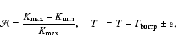
conductivity that corresponds to a bump in opacity. We recall below the temperature-dependent profile that is adopted for the radiative conductivity
are assumed to be constant. Following Paper I, the ionisation region is described by a parametric hollow in radiative
conductivity that corresponds to a bump in opacity. We recall below the temperature-dependent profile that is adopted for the radiative conductivity
 is the position of the hollow in temperature and
 ,
e and
,
e and  denote its slope, width and relative amplitude,
respectively.
denote its slope, width and relative amplitude,
respectively.
We are interested in small perturbations about the hydrostatic and radiative equilibria. The layer is fully radiative and the diffusion approximation implies that
Following Paper I, the depth d of the layer is selected as the length scale, and the top density
 and temperature
 as density and temperature scales, respectively. The velocity scale is thus
 .
Finally, gravity and fluxes are provided in units of
.
Finally, gravity and fluxes are provided in units of
 and
and
 ,
respectively. The linearised perturbations obey the following temperature, momentum and continuity dimensionless equations:
,
respectively. The linearised perturbations obey the following temperature, momentum and continuity dimensionless equations:
 denotes the density perturbation, u the velocity and
 the imposed bottom flux. Here we seek normal modes using a time-dependence of the form
 ,
with
,
with
 (
( is the damping or growth rate of the
mode and
is the damping or growth rate of the
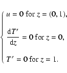
mode and  its frequency). Finally, by assuming rigid walls at both limits of the domain for the velocity, a perfect conductor at the bottom and a perfect insulator at the top for the temperature, we obtain the following boundary conditions
 is the eigenvalue associated with the (complex) eigenvector
 .
Here n defines the mode order, that is, the number of nodes of the eigenfunction u while the matrix A is a differential operator provided in Eq. (7), where the differential notation
.
Here n defines the mode order, that is, the number of nodes of the eigenfunction u while the matrix A is a differential operator provided in Eq. (7), where the differential notation
 is used for clarity
![\begin{figure}
\par\includegraphics[width=7.5cm,clip]{fig/9891fig1.eps} \end{figure}](/articles/aa/full/2008/41/aa09891-08/img48.gif) |
Figure 1:
Instability strip for the fundamental mode in the plane
 for
for
 and
and   10-4. The top (at z=1) density and temperature are
 10 -3 and T=1, respectively, while gravity is g=7 everywhere. The white cross denotes a particular simulation further studied for
 and
and
 . . |
| Open with DEXTER | |
Figure 1 displays the instability strip for the fundamental mode![[*]](/icons/foot_motif.gif) . In this parametric survey, we fix the slope
and width e of the conductivity hollow, whereas its amplitude
and temperature
vary (Eq. (1)). For every couple
,
both equilibrium fields and solutions to the eigenvalue problem (6) are completed using the LSB code (Linear Solver Builder, Valdettaro et al. 2007). Unstable modes with
. In this parametric survey, we fix the slope
and width e of the conductivity hollow, whereas its amplitude
and temperature
vary (Eq. (1)). For every couple
,
both equilibrium fields and solutions to the eigenvalue problem (6) are completed using the LSB code (Linear Solver Builder, Valdettaro et al. 2007). Unstable modes with  are identified
among all eigenvalues in each spectrum and only the fundamental mode is excited by the -mechanism in these simulations.
are identified
among all eigenvalues in each spectrum and only the fundamental mode is excited by the -mechanism in these simulations.
To confirm the reality of the instability strip and study the mode saturation, we perform a DNS of the nonlinear problem. We start from a linearly-unstable setup discovered in the parametric
survey (the white cross in Fig. 1 of which the oscillation spectrum is provided in Table 1) and advance hydrodynamic equations in time using the Pencil-Code.
Because we investigate the 1D case in this work, we cannot apply the 2D Alternate Direction Implicit (ADI) scheme developed in Paper I. We therefore code a 1D version of this scheme that consists of a
semi-implicit Crank-Nicholson algorithm where nonlinearities are dealt
with using a Jacobian factorisation (see e.g. Press et al. 1992, Sect. 16.6).
Table 1: First linear eigenvalues of the unstable setup used to start the DNS (this setup is denoted by the white cross in the instability strip in Fig. 1). Note that only the fundamental n=0 mode is linearly unstable.
![\begin{figure}
\par\includegraphics[width=8.4cm,clip]{fig/9891fig2.eps} \end{figure}](/articles/aa/full/2008/41/aa09891-08/img52.gif) |
Figure 2:
a) Temporal power spectrum for the momentum in the
 -plane. b) The resulting spectrum after integrating over depth. c) Comparison between normalised momentum profiles for -plane. b) The resulting spectrum after integrating over depth. c) Comparison between normalised momentum profiles for  modes according to the DNS power spectrum (solid black line) and to the linear-stability analysis (dotted blue line). modes according to the DNS power spectrum (solid black line) and to the linear-stability analysis (dotted blue line). |
| Open with DEXTER | |
To determine which modes are present in the DNS once it has reached the nonlinear-saturation regime, we perform in Fig. 2a a temporal Fourier transform of the momentum field
 and plot the power spectrum in the
-plane. With this method, acoustic modes are extracted because they emerge as ``shark fin profiles'' about definite eigenfrequencies (see Dintrans & Brandenburg 2004). In Fig. 2b, we integrate
and plot the power spectrum in the
-plane. With this method, acoustic modes are extracted because they emerge as ``shark fin profiles'' about definite eigenfrequencies (see Dintrans & Brandenburg 2004). In Fig. 2b, we integrate
 over depth to obtain the mean spectrum. Several discrete peaks corresponding to normal
modes appear but the fundamental mode close to
over depth to obtain the mean spectrum. Several discrete peaks corresponding to normal
modes appear but the fundamental mode close to
 clearly dominates.
The linear eigenfunctions can be compared to the mean profiles computed from a zoom about given eigenfrequencies in the DNS power spectrum shown in Fig. 2. Figure 2c displays such profiles about
and
 (solid black lines), whereas associated eigenfunctions are overplotted in dotted blue lines. The agreement between the linear-stability analysis and the DNS is remarkable.
In summary, Fig. 2 shows that several overtones are present in this DNS, even for long times. Because these overtones are linearly stable (see Table 1), some underlying energy transfers occur between modes. To investigate these intricate couplings in more detail, we need to follow the evolution of each mode separately using the projection method developed in the next section.
As said in the Introduction, the radiative diffusivity in our model is large close to the surface due to the instability criterion (the so-called ``transition region'' criterion). Eigenvectors
strongly differ from adiabatic ones, and therefore the quasi-adiabatic approximation fails in this case. The dissipative effects must be fully taken into account and the oscillations operator is non-Hermitian. In other words, the matrix A provided in Eq. (7) is not
self-adjoint and its eigenvectors
 are not mutually orthogonal. This implies that they cannot be used to arrange an acoustic subspace on which the physical fields of the DNS are projected. We thus consider the adjoint problem that has the same spectrum, while its
eigenvectors are orthogonal to A-ones because of the biorthogonality
property (see Appendix A.1).
are not mutually orthogonal. This implies that they cannot be used to arrange an acoustic subspace on which the physical fields of the DNS are projected. We thus consider the adjoint problem that has the same spectrum, while its
eigenvectors are orthogonal to A-ones because of the biorthogonality
property (see Appendix A.1).

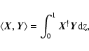
We start from the following inner-product
 denotes the Hermitian conjugate. The adjoint of the operator A is defined by (e.g. Löwdin 1983)
 of
of  are normalised to verify (see Appendix A.1)
 |
(10) |
are the eigenvectors of
such that
 |
(11) |
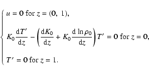
is provided in Eq. (16). This corresponds to the following
oscillation equations for the adjoint problem:
These boundary conditions are detailed in Appendix A.3. While integrating Eq. (A.6) by parts, we obtain surface contributions that must vanish to fulfill the adjoint definition (9) (Bohlius et al. 2007). This implies the following set
of adjoint boundary conditions
We solve the adjoint eigenvalue problem defined by Eqs. (12), (13) again using the LSB code, that is, we compute both the whole spectrum of eigenvalues
 and their associated eigenvectors
 .
An example is given in Fig. 3 where we plot the real part of both the regular (solid black line) and adjoint (dashed blue line) eigenfunctions of the fundamental n=0 mode.
.
An example is given in Fig. 3 where we plot the real part of both the regular (solid black line) and adjoint (dashed blue line) eigenfunctions of the fundamental n=0 mode.
![\begin{figure}
\par\includegraphics[width=8.2cm,clip]{fig/9891fig3.eps} \end{figure}](/articles/aa/full/2008/41/aa09891-08/img69.gif) |
Figure 3:
Real part of normalised eigenfunctions
 for the fundamental mode (solid black line) and its adjoint (dotted blue line), for the equilibrium setup denoted by a white cross in Fig. 1.
 |
| Open with DEXTER | |
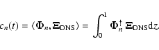
Once the two sets of (regular)
 and (adjoint)
eigenvector are known, the DNS fields are projected at each timestep using the following procedure:
and (adjoint)
eigenvector are known, the DNS fields are projected at each timestep using the following procedure:
 |
(14) |
 the temperature
and density perturbations provided by
the temperature
and density perturbations provided by
 |
(15) |
 |
(18) |
 by
by
![\begin{figure}
\par\includegraphics[width=8.4cm,clip]{fig/9891fig4.eps}\hspace*{0.4cm}
\includegraphics[width=8.2cm,clip]{fig/9891fig5.eps} \end{figure}](/articles/aa/full/2008/41/aa09891-08/img79.gif) |
Figure 4:
Left panel: time evolution of the real part of the complex-mode amplitudes cn(t) for
 modes. The theoretical growth or damping curves are overplotted in dashed blue lines. Right panel: their respective Fourier transforms. The modes eigenfrequencies are overplotted in dashed blue lines. modes. The theoretical growth or damping curves are overplotted in dashed blue lines. Right panel: their respective Fourier transforms. The modes eigenfrequencies are overplotted in dashed blue lines. |
| Open with DEXTER | |
The left panels of Fig. 4 show the time evolution of the real part of the projection coefficients cn(t) for the first four modes
.
We overplot the curves 
 derived from the linear-stability analysis (see
Table 1). As expected, only the fundamental mode amplitude c0(t) grows at each timestep. For other linearly-stable modes, amplitudes decay except for the n=2 one. The amplitude of this mode shows a transient decrease until time
derived from the linear-stability analysis (see
Table 1). As expected, only the fundamental mode amplitude c0(t) grows at each timestep. For other linearly-stable modes, amplitudes decay except for the n=2 one. The amplitude of this mode shows a transient decrease until time
 and then begins
to increase. This behaviour is an estimate of the nonlinear coupling that
occurs between this overtone and (at least) the fundamental mode.
and then begins
to increase. This behaviour is an estimate of the nonlinear coupling that
occurs between this overtone and (at least) the fundamental mode.
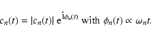
We next perform Fourier transforms of these mode amplitudes (right panel of Fig. 4). Following Eq. (19), the cn(t) amplitudes behave as
 because theoretical eigenfrequencies and peaks appearing in power spectra
overlap one another.
because theoretical eigenfrequencies and peaks appearing in power spectra
overlap one another.
![\begin{figure}
\par\includegraphics[width=8.4cm,clip]{fig/9891fig6.eps}\hspace*{0.3cm}
\includegraphics[width=8.2cm,clip]{fig/9891fig7.eps} \end{figure}](/articles/aa/full/2008/41/aa09891-08/img84.gif) |
Figure 5:
Phase diagrams for
modes. The abscissa (ordinate) corresponds to the real (imaginary) part of the complex mode amplitude cn(t). The increasing orbits are plotted in blue, whereas the decreasing ones are in black. |
| Open with DEXTER | |
In each panel of Fig. 5, the imaginary part of the complex mode amplitude cn(t) is plotted as a function of the real part for the four modes shown in Fig. 4. To avoid unreadable plots, we stop the time evolution at t=50. The decreasing orbits are plotted as black lines, whereas the increasing ones are in blue. In these diagrams, the radius of each trajectory is related to the modulus of the complex mode amplitude, which implies that a decreasing (increasing) radius is associated with a damped (excited) mode.
Once again, the fundamental mode appears to be continuously excited. We note that the excitation phenomenon is coherent in the sense that no discontinuity is observed in the mode orbits, that is, the spiral develops continuously. For the second overtone, after the linearly-transient decrease, the radius begins to increase significantly and this is still the signature of a nonlinear coupling with the fundamental mode. For the linearly-stable n=1 and n=3 modes, things are more intricate because a marginal increase is shown during the last orbits (also seen in Fig. 4). Unfortunately, these phase diagrams are not adapted to investigate this long-time dynamics because orbits will overlap one another.
To address the mode couplings responsible for the nonlinear limit-cycle stability observed at late times, we compute the energy content of each mode separately.
In BCM93, the total amount of sound generated by the turbulent convection is weak because they find that only  of the kinetic energy is stored in acoustic standing waves. Our problem
however consists of an initially static radiative zone without convection and the velocity field that develops is only due to acoustic modes, that is,
of the kinetic energy is stored in acoustic standing waves. Our problem
however consists of an initially static radiative zone without convection and the velocity field that develops is only due to acoustic modes, that is,
 |
(21) |
 and un are the velocity of the DNS and the regular eigenvector, respectively. By multiplying by
 ,
the kinetic energy density
,
the kinetic energy density
 is obtained as
 |
= | 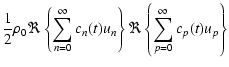 |
|
| = | ![$\displaystyle \displaystyle\sum_{n=0}^\infty \sum_{p=0}^\infty \frac{1}{2}\rho_0
\Re[c_n(t) u_n]\Re[c_p(t) u_p].$](/articles/aa/full/2008/41/aa09891-08/img93.gif) |
(22) |
![\begin{displaymath}%
E^{\rm tot}_{{\rm kin}}=\sum_{n=0}^\infty \left(\sum_{p=0}^...
...int_0^1\rho_0
\Re[c_n(t) u_n]\Re[c_p(t) u_p] {\rm d}z\right).
\end{displaymath}](/articles/aa/full/2008/41/aa09891-08/img94.gif) |
(23) |
![\begin{displaymath}%
E_n=\sum_{p=0}^\infty \frac{1}{2}\int_0^1\rho_0
\Re[c_n(t) u_n]\Re[c_p(t) u_p] {\rm d}z.
\end{displaymath}](/articles/aa/full/2008/41/aa09891-08/img95.gif) |
(24) |
 for
for
 .
After the transient linear growth of the
fundamental mode, a given fraction of energy is progressively transferred to upper overtones and the nonlinear saturation is achieved above
.
After the transient linear growth of the
fundamental mode, a given fraction of energy is progressively transferred to upper overtones and the nonlinear saturation is achieved above
 .
These nonlinear couplings mainly involve
the n=0 and n=2 modes because their energy ratios are dominant. However, the other overtones (i.e.
.
These nonlinear couplings mainly involve
the n=0 and n=2 modes because their energy ratios are dominant. However, the other overtones (i.e.
 )
also participate in this nonlinear saturation process but their energy ratios remain below
)
also participate in this nonlinear saturation process but their energy ratios remain below  .
This is compatible with the weak peaks around
the corresponding frequencies
shown in the power spectrum in Fig. 2b or with the marginal increase of the radius orbits in Fig. 5. It is at first glance not surprising because a high-order mode is associated with smaller scales and therefore with a high damping rate (Table 1). This implies that the excitation of these overtones from the fundamental mode would require efficient underlying couplings that are not observed in this
simulation.
.
This is compatible with the weak peaks around
the corresponding frequencies
shown in the power spectrum in Fig. 2b or with the marginal increase of the radius orbits in Fig. 5. It is at first glance not surprising because a high-order mode is associated with smaller scales and therefore with a high damping rate (Table 1). This implies that the excitation of these overtones from the fundamental mode would require efficient underlying couplings that are not observed in this
simulation.
![\begin{figure}
\par\includegraphics[width=8.3cm,clip]{fig/9891fig8.eps} \end{figure}](/articles/aa/full/2008/41/aa09891-08/img101.gif) |
Figure 6:
a) Kinetic energy ratios for
in a logarithmic y-scale. b) Zoom in the n=0 (solid black line) and n=2 (dashed green line) mode energy contents. |
| Open with DEXTER | |
The fact that the n=2 mode is more excited than the n=1 one nevertheless contradicts this explanation because its damping rate is more than twice the n=1 one. In Fig. 6b, we expand Fig. 6a for the fundamental mode and this second overtone only. The major energy transfer well occurs between these two modes because they contain about
of the total kinetic energy of this DNS. The reason for this favored coupling lies in the period ratio existing between these two modes (see Table 1): the fundamental period is
 ,
while the n=2 one is
,
while the n=2 one is
 such that the corresponding period ratio is
close to one half (
such that the corresponding period ratio is
close to one half (
 ). The n=2 mode therefore receives in a preferential way some energy from the n=0 mode every two periods and that corresponds, from a dynamical point
of view, to a classical 2:1 resonance. Such a resonance is usual in celestial mechanics with, e.g., Jupiter's moons Io (P=1.769 d), Europa (P=3.551 d) and Ganymede (P=7.154 d) and it is well
known that it helps to stabilise orbits. In our case, this stabilisation takes the form of a nonlinear saturation: the linear growth of the fundamental mode is balanced by the pumping of
energy from the linearly-stable second overtone behaving as an energy sink. The final amplitudes give about
). The n=2 mode therefore receives in a preferential way some energy from the n=0 mode every two periods and that corresponds, from a dynamical point
of view, to a classical 2:1 resonance. Such a resonance is usual in celestial mechanics with, e.g., Jupiter's moons Io (P=1.769 d), Europa (P=3.551 d) and Ganymede (P=7.154 d) and it is well
known that it helps to stabilise orbits. In our case, this stabilisation takes the form of a nonlinear saturation: the linear growth of the fundamental mode is balanced by the pumping of
energy from the linearly-stable second overtone behaving as an energy sink. The final amplitudes give about  of the kinetic energy in the fundamental mode and
  in the second overtone, the remaining 2 percent being in higher overtones as displayed in Fig. 6a.
The nonlinear saturation in our excitation model therefore results from a 2:1 resonance between the fundamental mode and the second overtone. As shown in the Introduction, this mechanism has also been proposed to explain the secondary bump observed in the luminosity variations of Bump Cepheids (SS76). An interesting correlation between the value of the ratio P2/P0 and the bump position was also emphasised leading to the so-called ``Hertzsprung progression'' (Buchler et al. 1990; Kovacs & Buchler 1989; Simon & Lee 1981). Nevertheless this correlation with P2/P0 is not observed as the period P2 deduced from luminosity curves is necessarily equal to P0/2. Indeed, the second overtone period changes due to nonlinear couplings and finally reaches the value P2= P0/2 once the nonlinear saturation is achieved (i.e. the 2:1 resonance). As a consequence, only linear eigenperiods are relevant when studying the influence of the P2/P0 ratio on the bump position. Furthermore, Buchler et al. (1990) have shown that this correlation between the phase and the P2/P0 ratio is not reproduced in their models when plotting the phase as a function of P0only. As our hydrodynamical model deals with dimensionless quantities, studying the phase variations according to P2/P0 is also more consistent.
![\begin{figure}
\par\includegraphics[width=7.5cm,clip]{fig/9891fig9.eps} \end{figure}](/articles/aa/full/2008/41/aa09891-08/img107.gif) |
Figure 7: P2/P0 level lines overplotted on the instability strip. Dashed white lines denote ratio P2/P0 <1/2, while solid white lines correspond to P2/P0 >1/2. The critical level P2/P0=1/2 is emphasised as a red line, and the dashed box delimits the region where a large number of DNS are performed to study Hertzsprung's progression (see Figs. 8, 9). |
| Open with DEXTER | |
To determine whether our model is able to reproduce this Hertzsprung progression, we first overplot in Fig. 7 the P2/P0 level lines with the instability strip discovered in the linear-stability analysis (Sect. 2.1). The solid white level lines correspond to
P2/P0 > 1/2, the dashed lines to
P2/P0 < 1/2 and the red line is for the critical level
P2/P0=1/2. The instability strip is clearly split in two separate parts and the most unstable modes belong to the
P2/P0<1/2 region. If we now perform the DNS corresponding to those different setups, we can check if the luminosity bump position is really correlated with the period ratio value. Because we are dealing with the 1D case, the luminosity reduces to the radiative flux at the top of the domain, that is,
 |
(25) |
 happen about
.
happen about
.
We then run a large number of DNS (up to 400) in the instability strip to cover a significant range in the P2/P0 ratio and cross the 1/2-line; all these DNS belong to the dashed box shown
in Fig. 7. In each case, the simulation is performed above the nonlinear saturation (
 ). Because we know that the fundamental mode and the second overtone enter in the time evolution of the emerging flux
,
we fit the obtained flux variations using the following decomposition:
). Because we know that the fundamental mode and the second overtone enter in the time evolution of the emerging flux
,
we fit the obtained flux variations using the following decomposition:
![$[A_0,\ A_2,\ \phi_0,\ \phi_2]$](/articles/aa/full/2008/41/aa09891-08/img112.gif) are computed using the Levenberg-Marquardt algorithm that is a nonlinear least-square method (e.g. Press et al. 1992, Sect. 15.5). The phase shift between the two signals is defined by
are computed using the Levenberg-Marquardt algorithm that is a nonlinear least-square method (e.g. Press et al. 1992, Sect. 15.5). The phase shift between the two signals is defined by
 is less (greater) than
  ,
this secondary bump will be located in
the descending (ascending) branch after (before) the flux maximum.
,
this secondary bump will be located in
the descending (ascending) branch after (before) the flux maximum.
The whole DNS are summarised in Fig. 8 where isocontours of
are plotted in the same
instability strip plane used in Fig. 7. The
red regions are associated with
 ,
the blue ones with
,
the blue ones with
 and the white ones with
 .
By overplotting the level lines of the period ratio P2/P0, the following correspondence appears:
.
By overplotting the level lines of the period ratio P2/P0, the following correspondence appears:
![\begin{figure}
\par\includegraphics[width=7.5cm,clip]{fig/9891fig10.eps} \end{figure}](/articles/aa/full/2008/41/aa09891-08/img119.gif) |
Figure 8:
Isocontours of
in the
plane (note that we rather plot
 to highlight the critical line
). This figure corresponds to the dashed box in Fig. 7 and the black circles display eleven
selected simulations showed in Fig. 9.
to highlight the critical line
). This figure corresponds to the dashed box in Fig. 7 and the black circles display eleven
selected simulations showed in Fig. 9. |
| Open with DEXTER | |
![\begin{figure}
\includegraphics[width=8.3cm,clip]{fig/9891fig11.eps} \end{figure}](/articles/aa/full/2008/41/aa09891-08/img120.gif) |
Figure 9: Rephased time evolutions of the surface radiative flux about time t=500 for the eleven selected simulations plotted as black circles in Fig. 8. The ratio of eigenperiods P2/P0 is indicated in each case. |
| Open with DEXTER | |
To highlight this result, examples of light curves shaping an Hertzsprung progression are provided in Fig. 9. These eleven curves correspond to the black circles distributed across the P2/P0=1/2 level line in Fig. 8. The correspondences (28) appear clearly: the bump is located in the descending branch of the light curve if P2/P0 > 1/2, while values P2/P0 <1/2 lead to a bump in the ascending branch.
Observations also show that the amplitude of the surface velocity presents a double-peaked behavior along the Hertzsprung progression as its center corresponds to a minimum value for the velocity (Bono et al. 2000). In our simulations, no clear correlation between the amplitude ratio A2/A0 and the bump position appears and we guess that it may be related to the two following restrictions:
 ,
there are not enough variations to obtain significant changes in this ratio.
,
there are not enough variations to obtain significant changes in this ratio.
In this paper, we investigate the nonlinear saturation of the acoustic modes excited by the -mechanism in direct numerical simulations (DNS). This study follows on from our former work where we began our modelling of the -mechanism in Cepheids by looking the propagation of
acoustic modes in a layer of gas in which the ionisation is modelled by a hollow in the radiative conductivity profile (Gastine & Dintrans 2008, Paper I).
To catch the evolution of linearly-unstable modes, we apply an original method consisting of the projection of the DNS fields onto the eigenmodes that are solutions to the linear oscillation equations (Dintrans & Brandenburg 2004). Because the oscillation operator is non-Hermitian, the regular eigenvectors are not mutually orthogonal and we consider the adjoint problem that has the same spectrum while its eigenvectors are orthogonal to the regular ones. Thanks to these two sets of eigenvectors, we compute the projection coefficients for each DNS snapshot and follow the temporal evolution of acoustic modes separately. Corresponding phase diagrams show that the orbit radius of the linearly-unstable fundamental mode is continuously growing with time. On the contrary, orbits associated with the linearly-stable overtones exhibit decreasing radii, except the n=2 one that is increasing at late times.
We derive the kinetic energy contributions of each mode propagating in the DNS. More than
of the total kinetic energy is contained in two modes corresponding to the fundamental
mode and the second overtone. This last mode, which represents about  of the total kinetic energy, is involved in the nonlinear saturation of the instability through a 2:1 resonance with the fundamental mode. It means that the unstable fundamental mode gives energy to the stable second overtone that leads to the limit-cycle stability, as displayed in Fig. 6.
This 2:1 resonance is striking because the same mechanism is probably responsible for the observed bump in the luminosity curves of Bump Cepheids, leading to the well-known ``Hertzsprung's progression''. This progression links the bump position to the period ratio P2/P0 existing between the fundamental mode and the second overtone (SS76). We perform a large number of DNS covering a significant range in this ratio and extract the resulting luminosity curves. The 2:1 resonance does lead to an Hertzsprung progression as the bump arises in the ascending branch for P2/P0 < 1/2, while it is located in the descending branch for P2 /P0 > 1/2.
The study of the -mechanism in a purely-radiative layer is now completed with this work. The physical criteria for the instability as well as the nature of its nonlinear saturation are addressed. Future works will be devoted to the influence of convection on the mode stability. Indeed, a coupling between the convection and pulsations is suspected to play a major role in the disappearance of unstable modes close to the red edge of Cepheids' instability strip.
Time-dependent theories of convection have difficulty in explaining the red-edge location since they rely on many unconstrained parameters (e.g. Wuchterl & Feuchtinger 1998; Yecko et al. 1998). Because DNS fully account for
crucial nonlinearities, they are appropriate to properly investigate this dynamical coupling between the acoustic modes and convection. We thus plan to perform 2D DNS of the -mechanism in the presence of convection. The interesting cases will of course correspond to a (local)
convective-turnover timescale of the same order as the period of the fundamental mode.
Acknowledgements
We thank the referee (G. Bono) for his fruitful comments. Calculations were carried out on the CalMip machine of the ``Centre Interuniversitaire de Calcul de Toulouse'' (http://www.calmip.cict.fr/) and Grid'5000, which is an initiative from the French Ministry of Research through the ACI GRID incentive action, INRIA, CNRS and RENATER and other contributing partners (see https://www.grid5000.fr).
We consider a continuous linear operator H with eigenvalues  and eigenvectors
 linked by
 |
(A.1) |
 is its adjoint with eigenvalues
  and eigenvectors
as
and eigenvectors
as
 |
(A.2) |
 |
(A.3) |
 |
(A.4) |
The relation (9) that links an operator with its adjoint takes the following form in our problem
 is an adjoint eigenvector and
 is a regular one. To determine the adjoint operator ,
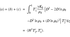
we calculate each element successively from the regular matrix in Eq. (7). We provide below an example of
such a calculation for the first column of the adjoint matrix given in Eq. (16).
is a regular one. To determine the adjoint operator ,
we calculate each element successively from the regular matrix in Eq. (7). We provide below an example of
such a calculation for the first column of the adjoint matrix given in Eq. (16).
 Calculation of

comes from the following inner-product
![\begin{displaymath}%
I \!=\! \langle T'_{2}, A_{11} T'_1 \rangle
\! =\! \displa...
..._0}\left[K_0 D^2\!+\!2DK_0
D \!+\!D^2
K_0\right]T'_1 {\rm d}z.
\end{displaymath}](/articles/aa/full/2008/41/aa09891-08/img137.gif) |
(A.7) |
| I | = | 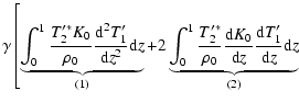 |
|
![$\displaystyle \left.+ \underbrace{\int_0^1\frac{T'^*_2}{\rho_0}\frac{{\rm d}^2 K_0}{{\rm d}z^2}T'_1
{\rm d}z}_{(a)}\right].$](/articles/aa/full/2008/41/aa09891-08/img139.gif) |
(A.8) |
 |
(A.11) |
Calculation of

comes from the following inner-product
![\begin{displaymath}%
\langle T'_{2}, A_{12} u_1 \rangle = \int_0^1
T'^*_{2}\left[\frac{F_{{\rm bot}}}{K_0}-(\gamma-1)T_0 D\right]u_1 {\rm d}z.
\end{displaymath}](/articles/aa/full/2008/41/aa09891-08/img144.gif) |
(A.12) |
![\begin{displaymath}%
\begin{array}{rcl}
\langle T'_{2}, A_{12} u_1 \rangle &=& ...
...e{(\gamma-1)\left[ T'^*_2 T_0 u_1\right]_0^1}_{=0}.
\end{array}\end{displaymath}](/articles/aa/full/2008/41/aa09891-08/img145.gif) |
(A.13) |
 |
(A.14) |
Calculation of

Because A13=0 in Eq. (7), we have
 |
(A.15) |
 |
(A.16) |
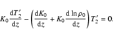
To determine the boundary conditions for the adjoint problem, we follow a method used in Bohlius et al. (2007). Equation (A.9) contains the boundary conditions on
temperature because the definition of the adjoint operator (9) imposes that every integrated term vanishes as
![\begin{displaymath}%
\begin{array}{rcl}
(1)+(2) &= & \displaystyle \left[\frac{...
...rac{T'^*_2 K_0}{\rho_0}\right)T'_1\right
] _0^1 =0.
\end{array}\end{displaymath}](/articles/aa/full/2008/41/aa09891-08/img150.gif) |
(A.17) |
![\begin{displaymath}%
\left[2\frac{T'^*_2}{\rho_0}\frac{{\rm d} K_0}{{\rm d}z}-\f...
...rm d}z}\left(
\frac{T'^*_2 K_0}{\rho_0} \right)\right]T'_1=0,
\end{displaymath}](/articles/aa/full/2008/41/aa09891-08/img152.gif) |
(A.19) |
![\begin{displaymath}%
K_0(T)=K_{{\rm max}}\left[1+{\cal A}\frac{-\pi/2+\arctan(\sigma
T^+T^-)}{\pi/2+\arctan(\sigma e^2)}\right],
\end{displaymath}](/articles/aa/full/2008/41/aa09891-08/img24.gif)